---
title: Survival Analysis with the Kaplan-Meier Method
description: "Walk through a Kaplan-Meier survival analysis step by step: estimate survival curves, compare groups with RMST, and interpret the results. Uses built-in sample data so you can follow along in your browser without installing anything."
priority: 0.6
---
# Tutorial: Survival Analysis with the Kaplan-Meier Method {#tutorial-kaplan-meier-survival-curves-with-heart-failure-data}
This tutorial walks through a Kaplan-Meier survival analysis from start to finish, using heart failure clinical records included as sample data in MIDAS. No installation or coding is needed — everything runs in your browser. [Open the sample data in MIDAS](../shared/files/tutorial-kaplan-meier-data.mds) to follow along.
You have clinical records for 299 patients diagnosed with heart failure, tracking their survival status over a follow-up period. In this tutorial, you will estimate survival curves using the Kaplan-Meier method and compare survival curves grouped by patient characteristics (anaemia, high blood pressure) using RMST (Restricted Mean Survival Time).
1. Load the sample data and examine its structure
2. Understand the key feature of survival data: censoring
3. Estimate the overall survival curve
4. Compare survival curves between patients with and without anaemia
5. Interpret the RMST results
6. Explore other grouping variables
## Load the data {#load-the-data}
On the launcher screen, click **Heart Failure** in the Sample Data section. A project is created and the data is loaded.
[Open this state in MIDAS](../shared/files/tutorial-kaplan-meier-data.mds)
This dataset contains clinical records of heart failure patients collected at the Faisalabad Institute of Cardiology (Pakistan) in 2015 ([Chicco & Jurman, 2020](#ref-chicco-jurman-2020)).
## Examine the data structure {#examine-the-data-structure}
Open the Data Table tab. You will see 299 rows and 13 columns.
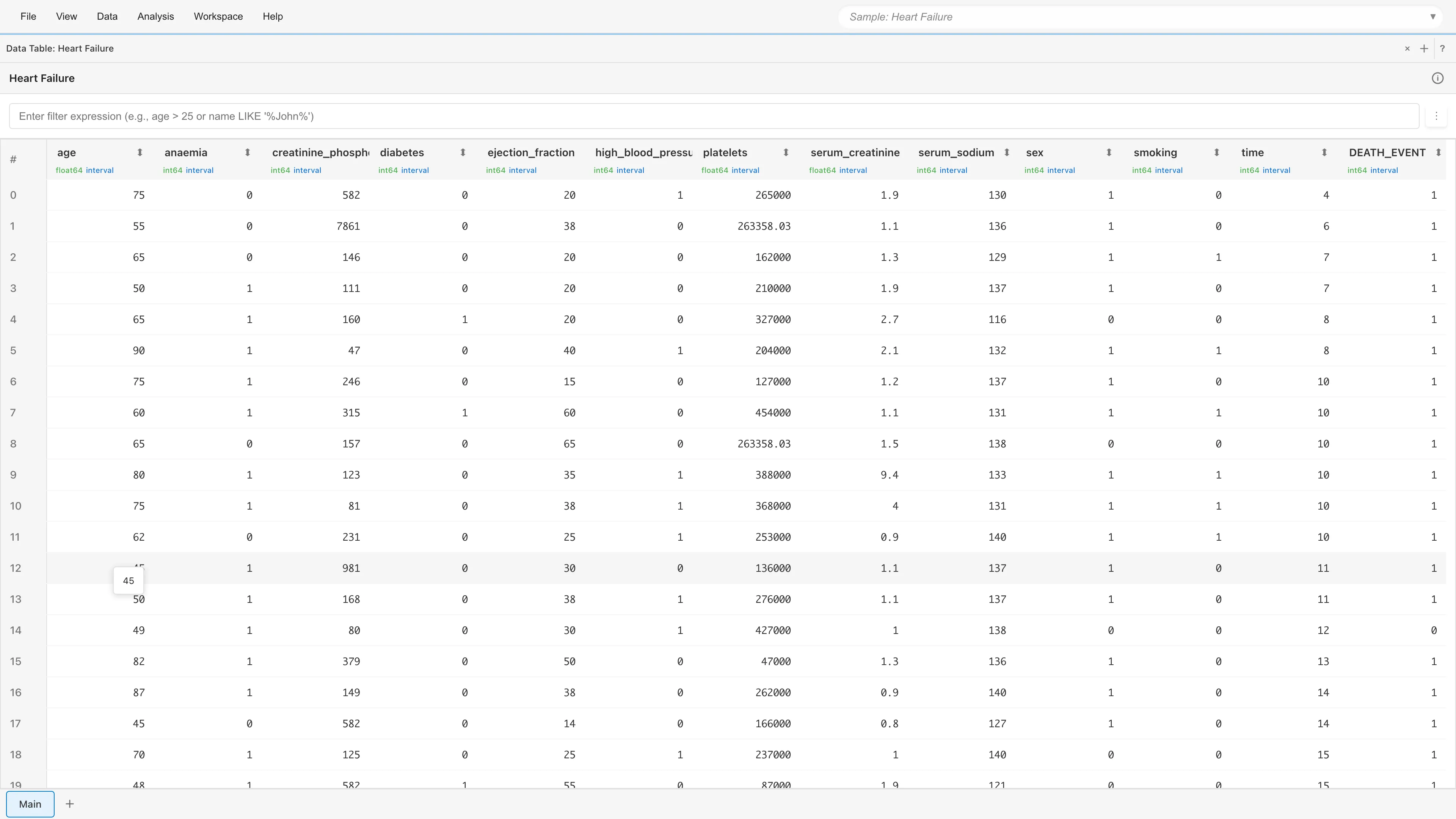
The key columns for survival analysis fall into three categories.
### Time and event variables {#time-and-event-variables}
| Column | Description |
|--------|-------------|
| `time` | Follow-up period in days. The number of days from diagnosis to the last observation (death or censoring) |
| `DEATH_EVENT` | Whether the patient died during follow-up. 1 = death, 0 = alive ([censored](#what-is-censoring)) |
### Patient characteristics (used for grouping) {#patient-characteristics-used-for-grouping}
| Column | Description |
|--------|-------------|
| `age` | Age in years |
| `anaemia` | Presence of anaemia (0: No, 1: Yes) |
| `diabetes` | Presence of diabetes (0: No, 1: Yes) |
| `high_blood_pressure` | Presence of hypertension (0: No, 1: Yes) |
| `sex` | Sex (0: Female, 1: Male) |
| `smoking` | Smoking status (0: No, 1: Yes) |
### Laboratory values {#laboratory-values}
The remaining 5 columns (`creatinine_phosphokinase`, `ejection_fraction`, `platelets`, `serum_creatinine`, `serum_sodium`) are blood test results. They are not used in this tutorial but can serve as covariates in Cox regression.
## What is censoring? {#what-is-censoring}
Of the 299 patients, some died during follow-up (`DEATH_EVENT = 1`) and others were still alive when follow-up ended (`DEATH_EVENT = 0`). The latter are called **censored** observations.
A censored patient's survival time is at least `time` days, but when the event will eventually occur is unknown.
If you simply excluded censored patients, you would lose the information from patients who survived for long periods without an event, estimating survival times only from those who died. This underestimates survival. The Kaplan-Meier method accounts for censoring by incorporating the "survived at least this long" information into the risk set calculation.
For this estimation to be valid, censoring must be independent of the likelihood of experiencing the event (non-informative censoring). For the mathematical treatment of censoring, see [Survival Analysis Fundamentals](concepts-survival#time-to-event-data-and-censoring).
## Estimate the overall survival curve {#estimate-the-overall-survival-curve}
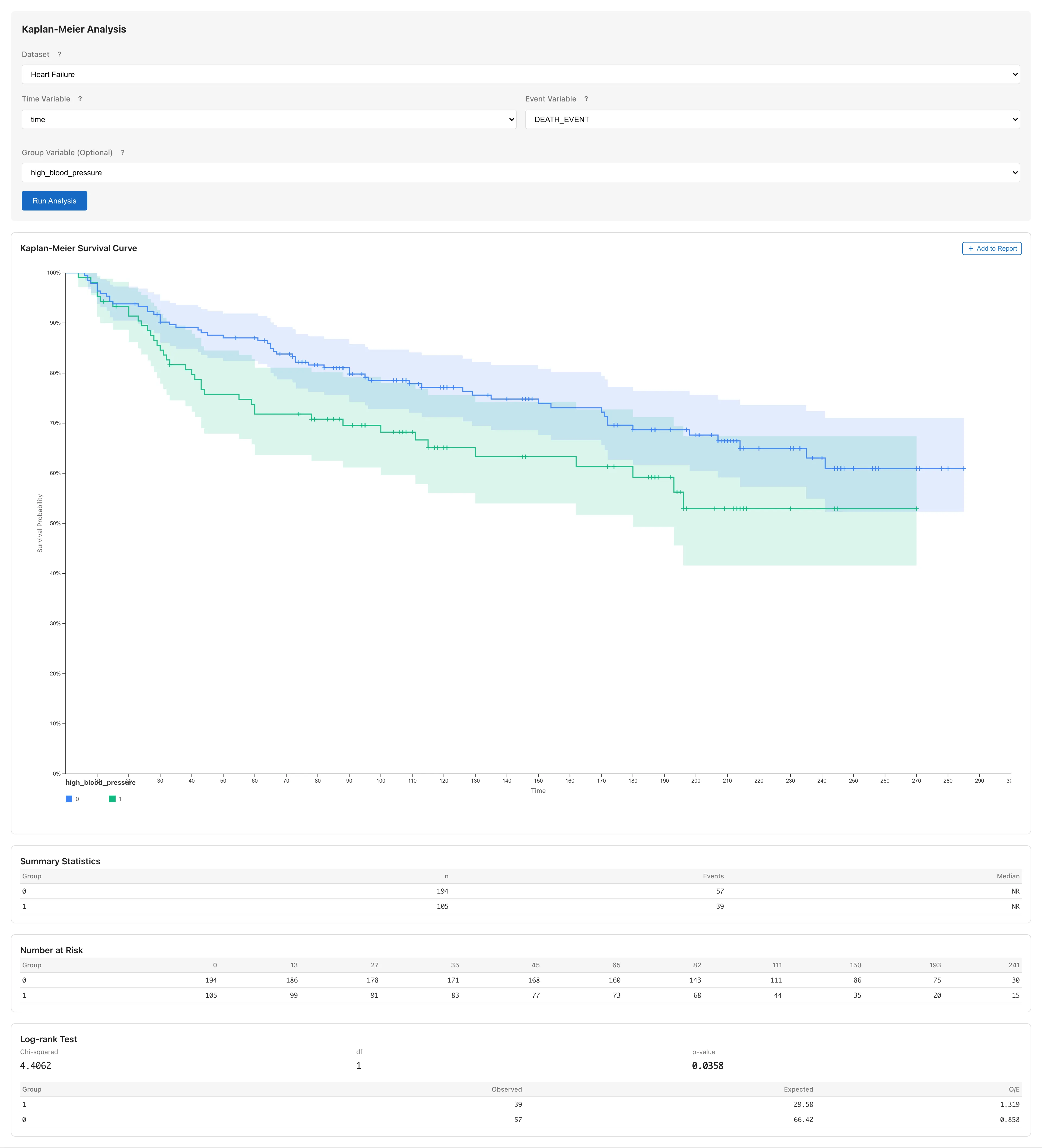
Select **Analysis > Survival Analysis > Kaplan-Meier...** from the menu bar. The Kaplan-Meier tab opens.
### Set variables {#set-variables}
- **Time Variable**: select `time`
- **Event Variable**: select `DEATH_EVENT`
Leave **Group Variable (Optional)** empty.
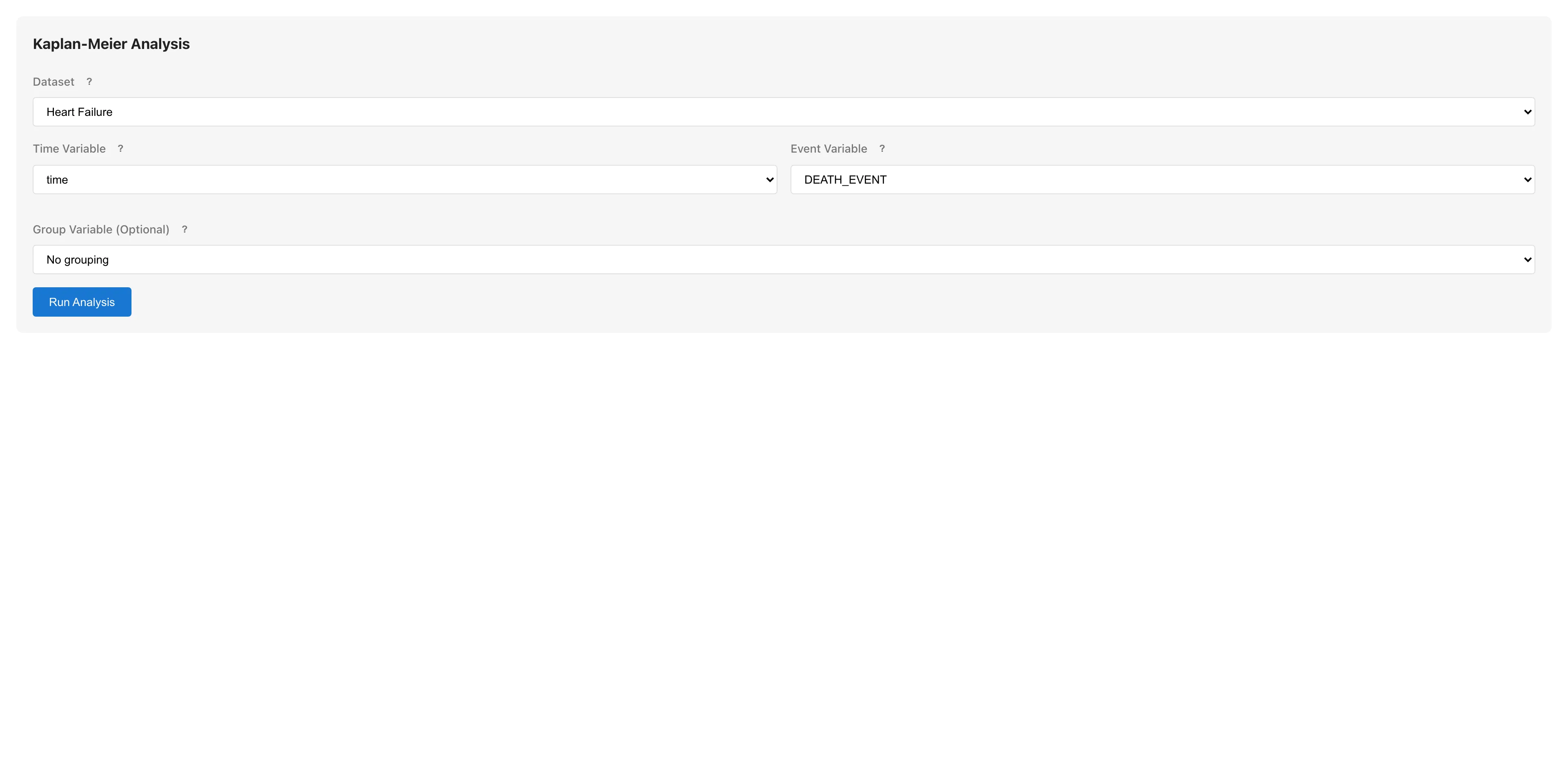
Click **Run Analysis**.
[Open this state in MIDAS](../shared/files/tutorial-kaplan-meier-overall.mds)
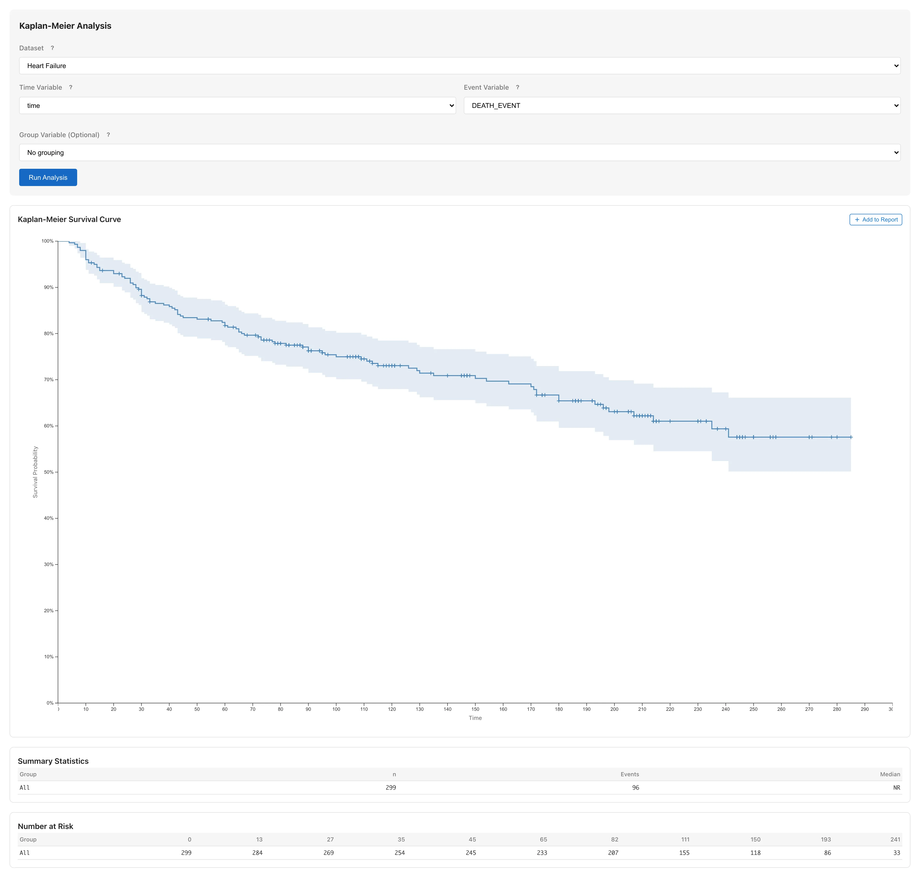
### Read the survival curve {#read-the-survival-curve}
The horizontal axis shows follow-up time (days) and the vertical axis shows survival probability $S(t)$. The Kaplan-Meier method does not assume a distributional form — it estimates survival probability directly at each event time, producing a step function that drops when a death occurs. The + marks on the curve indicate censoring times — points where subjects were lost to follow-up. The shaded band around the curve is the 95% confidence interval for the estimated survival probability $S(t)$ at each time point (a pointwise interval constructed independently at each time, not a simultaneous band covering the entire curve).
### Check Summary Statistics {#check-summary-statistics}
| Item | Meaning |
|------|---------|
| n | Number of subjects (299) |
| Events | Number of deaths |
| Median | Median survival time |
| 95% CI | Confidence interval for the median |
The median is the time point where the survival curve crosses the $S(t) = 0.5$ line. It represents when half of the subjects have experienced the event, and is widely used as a summary measure of survival. If $S(t)$ does not fall below 0.5 within the observation period, the median is displayed as NR (Not Reached).
## Compare survival curves by anaemia status {#compare-survival-curves-by-anaemia-status}
Next, examine whether survival differs between patients with and without anaemia.
### Set the Group Variable {#set-the-group-variable}
Select `anaemia` from the **Group Variable (Optional)** dropdown and click **Run Analysis**.
[Open this state in MIDAS](../shared/files/tutorial-kaplan-meier-anaemia.mds)
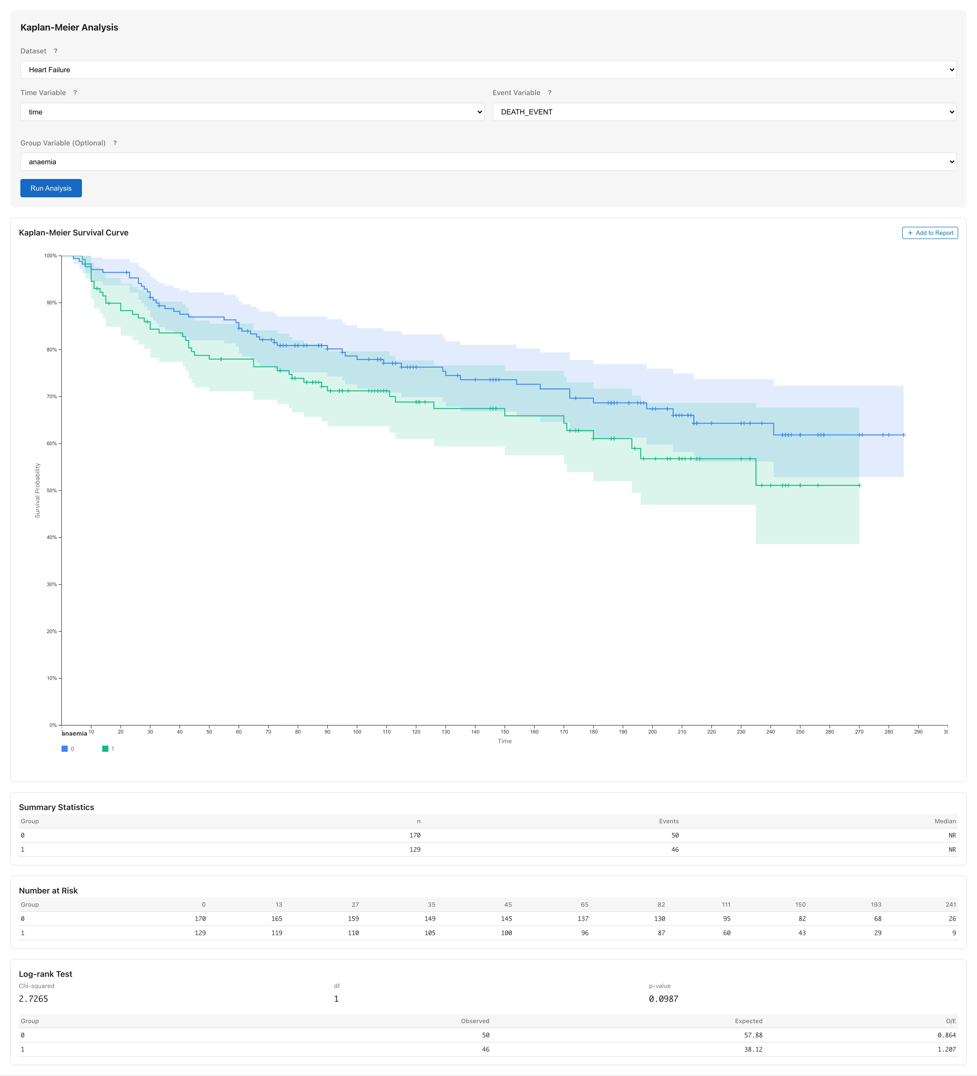
Two survival curves appear: `anaemia = 0` (no anaemia) and `anaemia = 1` (anaemia present).
### Read the curves {#read-the-curves}
The gap between the two curves at each time point is the estimated difference in survival probability between groups. The confidence bands represent the estimation precision of each group's survival function; overlap between bands does not indicate whether the groups differ, because each band is constructed independently for that group and has a different structure from a confidence interval for the difference. Use RMST to compare groups quantitatively.
### Interpret the RMST results {#interpret-the-rmst}
Below the curves, the RMST (Restricted Mean Survival Time) results appear for each group.
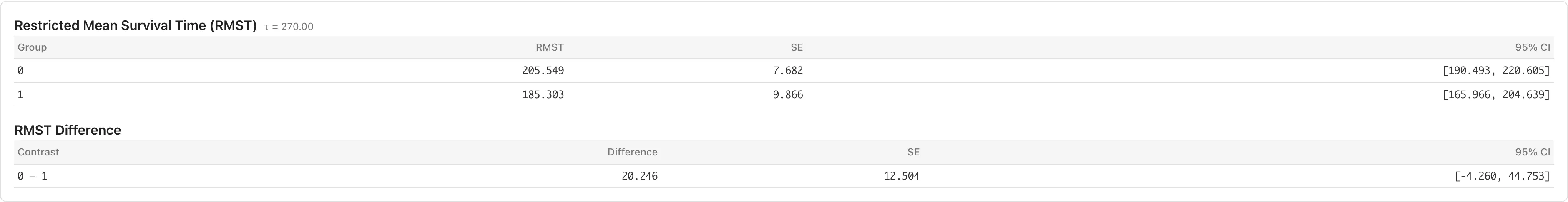
RMST is the area under the Kaplan-Meier curve from 0 to a restriction time $\tau$, estimating the average survival time up to $\tau$. RMST does not require the proportional hazards assumption and remains interpretable even when survival curves cross ([details](survival-analysis#rmst)).
| Column | Description |
|--------|-------------|
| Group | Group name |
| RMST | Restricted mean survival time estimate. Computed as the area under the KM curve up to $\tau$ |
| SE | Standard error, based on the Greenwood variance |
| 95% CI | 95% confidence interval for RMST |
When there are two or more groups, an **RMST Difference** table appears below. It shows the pairwise difference in RMST, its SE, and confidence interval. Read the magnitude of the difference and its uncertainty from the point estimate and the width of the confidence interval. For example, if the estimated difference is 15 days with a 95% CI of [3, 27], the average survival time up to $\tau$ is estimated to differ by approximately 15 days, and the range from 3 to 27 days represents the uncertainty of that estimate. For three or more groups, the table heading changes to **RMST Difference (Unadjusted)** and the per-pair confidence intervals are unadjusted for multiplicity.
### Number at Risk table {#number-at-risk-table}
The Number at Risk table below the curve shows how many patients remain in the risk set (neither dead nor censored) at each time point.
The numbers decrease over time as patients leave the risk set through both death and censoring. At time points where few patients remain, the survival estimate becomes less precise and the confidence band widens.
## Compare by other variables {#compare-by-other-variables}
Follow the same steps to compare by high blood pressure (`high_blood_pressure`) or smoking (`smoking`).
You can compute RMST with different group variables, but trying multiple grouping variables is hypothesis generation. Report findings from exploration as exploratory analysis.
Kaplan-Meier can only handle one grouping variable at a time. To consider multiple factors simultaneously, use the Cox proportional hazards model. For example, you can assess the effect of anaemia on survival while accounting for differences in age. See [Survival Analysis](survival-analysis#cox-regression) for instructions.
## Add results to a report {#add-results-to-a-report}
To save the survival curve for a paper or presentation, click the **Add to Report** button. In the dialog that appears, select an existing report or create a new one, and the survival curve is added to that report.
See [Reports](report) for details on working with reports.
## Summary {#summary}
- **Survival data structure**: You need a time variable (follow-up period) and an event variable (death/censoring)
- **Censoring**: Patients alive at the end of follow-up are included in the analysis as "survived at least this long"
- **Survival curve estimation**: The Kaplan-Meier method estimates the survival curve directly from observed data without assuming a distribution
- **Group comparison**: Setting a Group Variable produces group-specific survival curves and enables comparison via RMST differences
For the mathematical background of survival analysis, see [Survival Analysis Fundamentals](concepts-survival).
## References {#references}
- Chicco, D., & Jurman, G. (2020). Machine learning can predict survival of patients with heart failure from serum creatinine and ejection fraction alone. *BMC Medical Informatics and Decision Making*, 20, 16. https://doi.org/10.1186/s12911-020-1023-5
- Kaplan, E. L., & Meier, P. (1958). Nonparametric estimation from incomplete observations. *Journal of the American Statistical Association*, 53(282), 457-481. https://www.jstor.org/stable/2281868