Tutorial: Grouped Binomial GLM with Dose-Response Data

An insecticide is applied to groups of insects at increasing concentrations, and the number of deaths at each concentration is recorded. This tutorial fits a grouped binomial GLM (logistic regression) to that data and estimates how much the mortality rate increases per unit of concentration.

This tutorial uses dose-response data, but the same method applies to any data with the structure "K successes out of N trials at a given condition" — quality inspection pass/fail counts, epidemiological incidence data, and similar datasets.

The analysis proceeds as follows:

1. Load the sample data and examine its structure
2. Understand the difference between Binary and Grouped formats
3. Log-transform the predictor variable
4. Configure and run a Grouped Binomial GLM in the GLM tab
5. Read the coefficients table and Model Summary
6. Check diagnostic plots to assess model adequacy

Load the data

Click Dose Response in the Sample Data section on the launcher screen. A project is created and the data is loaded.

Open this state in MIDAS

This is synthetic data inspired by the classic beetle mortality experiment of Bliss (1935). At each of 8 concentration levels, approximately 50 insects are exposed, and the number of deaths is recorded.

Examine the data

Open the Data Table tab to see the 8-row, 4-column dataset.

Column	Description
dose	Insecticide concentration in mg/L, ranging from 1.0 to 128.0, roughly doubling at each step
exposed	Number of insects exposed at that concentration, between 46 and 52 per group
dead	Number of insects that died
mortality_rate	Mortality rate (dead / exposed), included for reference but not used in the analysis

The full dataset:

dose	exposed	dead	mortality_rate
1.0	50	1	0.020
2.0	48	3	0.063
4.0	46	8	0.174
8.0	50	28	0.560
16.0	47	42	0.894
32.0	52	49	0.942
64.0	49	47	0.959
128.0	51	50	0.980

The mortality_rate column shows 2% mortality at 1.0 mg/L, rising to 98% at 128.0 mg/L. Plotting with a log-scaled x-axis reveals a sigmoidal (S-shaped) pattern. Logistic regression models this S-curve.

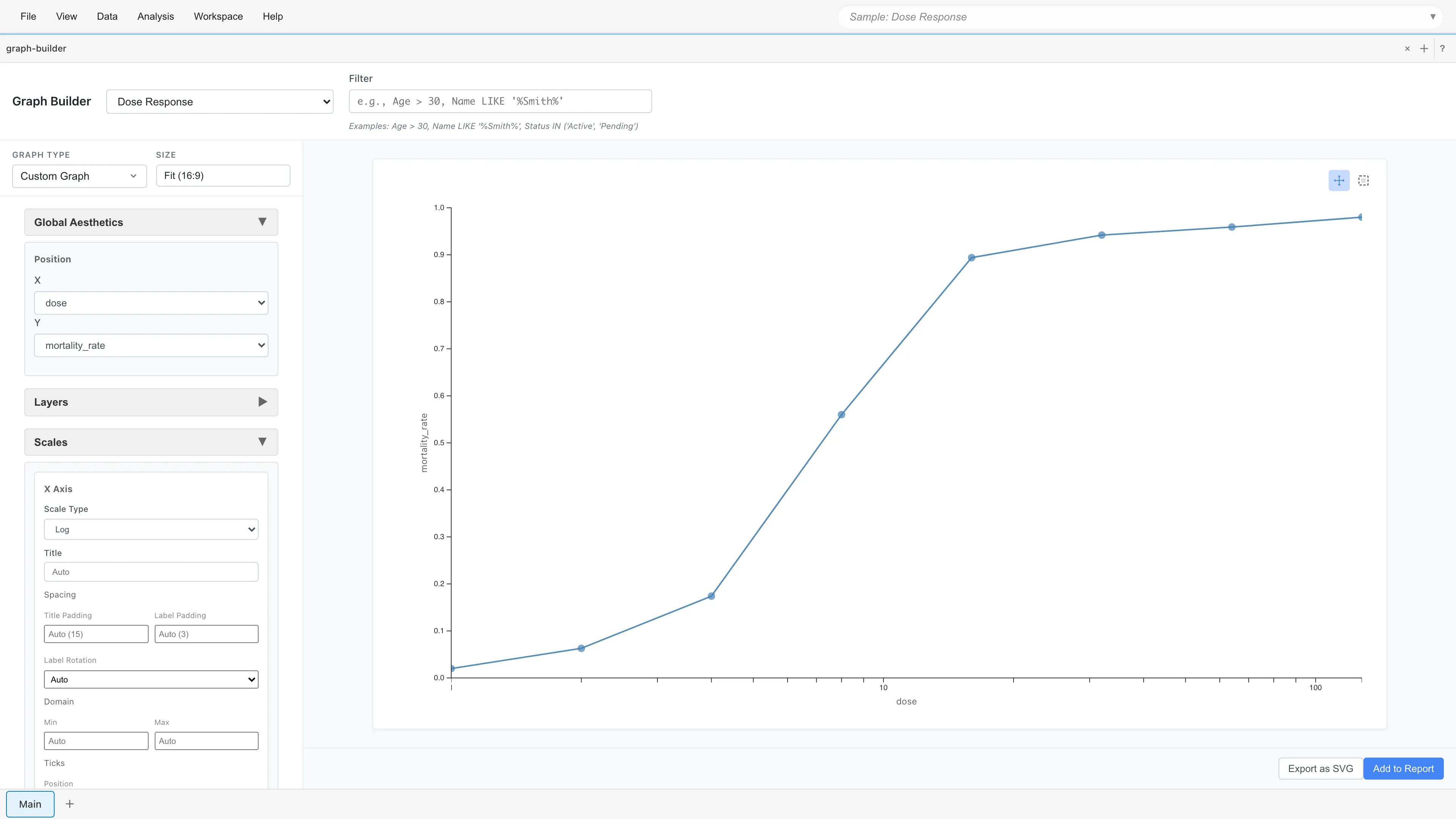
The key observation is that each row represents "how many out of how many died at a given concentration," not "whether a single insect died." This format is called Grouped format.

Binary vs Grouped

Binomial GLM supports two data formats.

Binary format uses one row per individual. Representing 3 deaths out of 50 insects requires 50 rows, each recording death = 1 or survival = 0. This format is used when individual-level covariates are available, such as patient-level clinical trial data.

Grouped format uses one row per condition. The same data is represented as dead = 3, exposed = 50 in a single row. Dose-response experiments, quality inspection pass rates, and epidemiological incidence data naturally come in this format.

When individuals within a condition are homogeneous (no individual-level covariates), both formats fit mathematically the same model. In grouped format, the response is the proportion $y = k/n$ (successes/trials), with trials $n$ passed as weights to the estimation engine. Since this data is aggregated by condition (concentration), grouped format is appropriate.

Log-transform the predictor

As the scatter plot showed, the relationship between dose and mortality_rate is sigmoidal on the log scale. GLM assumes a linear relationship between log-odds and the predictor, so using raw dose violates this assumption. The logarithm of dose should be used as the predictor.

Select Data > Add Columns.... The Add Columns tab opens.

• Enter log_dose in the Column name field
• Enter ln(dose) in the SQL expression field

Click Preview to check the result, then click Save. A new dataset is created with the log_dose column added to the original data.

Open this state in MIDAS

Open the GLM tab

Select Analysis > Generalized Linear Model (GLM)... from the menu bar. The GLM tab opens.

Select the dataset

In the Dataset dropdown, select the derived dataset created by Add Columns.

Configure the distribution family

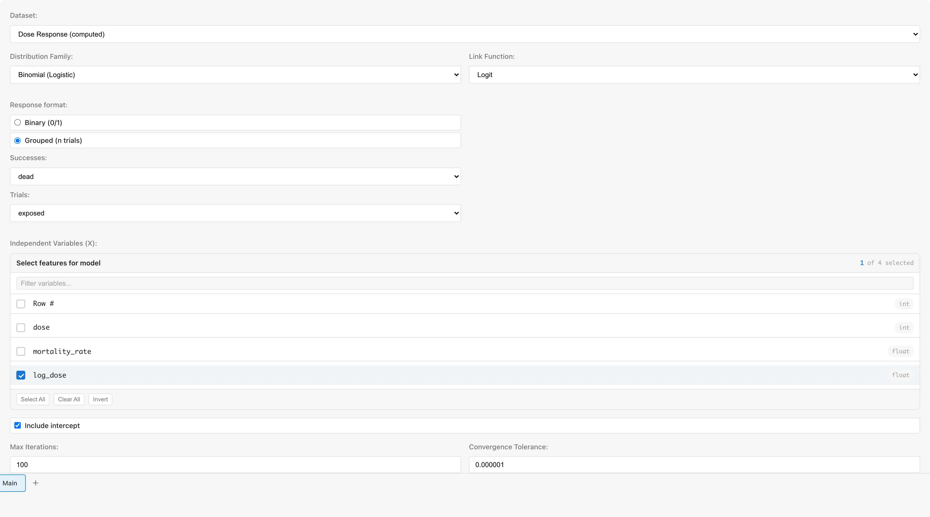
Set Distribution Family to Binomial (Logistic).

When Binomial is selected, a Response format option appears. The default is Binary (0/1). Since this is aggregated data, select Grouped (n trials).

After selecting Grouped, two dropdowns appear: Successes and Trials.

• Successes: Select dead. The number of deaths is the event of interest
• Trials: Select exposed. The number of insects exposed is the number of trials

MIDAS uses this specification to internally convert the response to $y = \text{dead} / \text{exposed}$ (mortality rate) and use the trial count exposed as weights for estimation.

Select predictor variables

Check log_dose under Independent Variables (X).

Leave Link Function at the default Logit.

The link function determines how to transform a probability into something a regression equation can work with. The mortality rate (probability $p$) is bounded between 0 and 1, but the regression equation $\beta_0 + \beta_1 \times \text{log\_dose}$ can produce any value from $-\infty$ to $+\infty$. These ranges do not match.

The logit link bridges this gap. It converts the probability $p$ into the odds $p / (1-p)$ (the ratio "probability of death / probability of survival"), then takes the logarithm. This $\log(p/(1-p))$ is called the log-odds (logit). Log-odds ranges from $-\infty$ to $+\infty$, so it can be directly connected to the regression equation.

Logit is the default link function for the Binomial family. There is no need to change it unless you have a specific reason.

Leave Include intercept checked.

Open this state in MIDAS

Run the analysis

Click Run GLM. A progress dialog shows the deviance at each iteration. With only 8 rows, this completes in a few seconds. Click OK when the completion dialog appears.

What is deviance? Deviance measures how much the model fails to explain the data — it plays a role analogous to the residual sum of squares in OLS regression (and equals it for the Gaussian family). Smaller values mean better fit. If deviance decreases at each iteration, the estimation is progressing normally.

Read the Model Summary

Open this state in MIDAS

The Model Summary appears at the top of the results.

Metric	Meaning
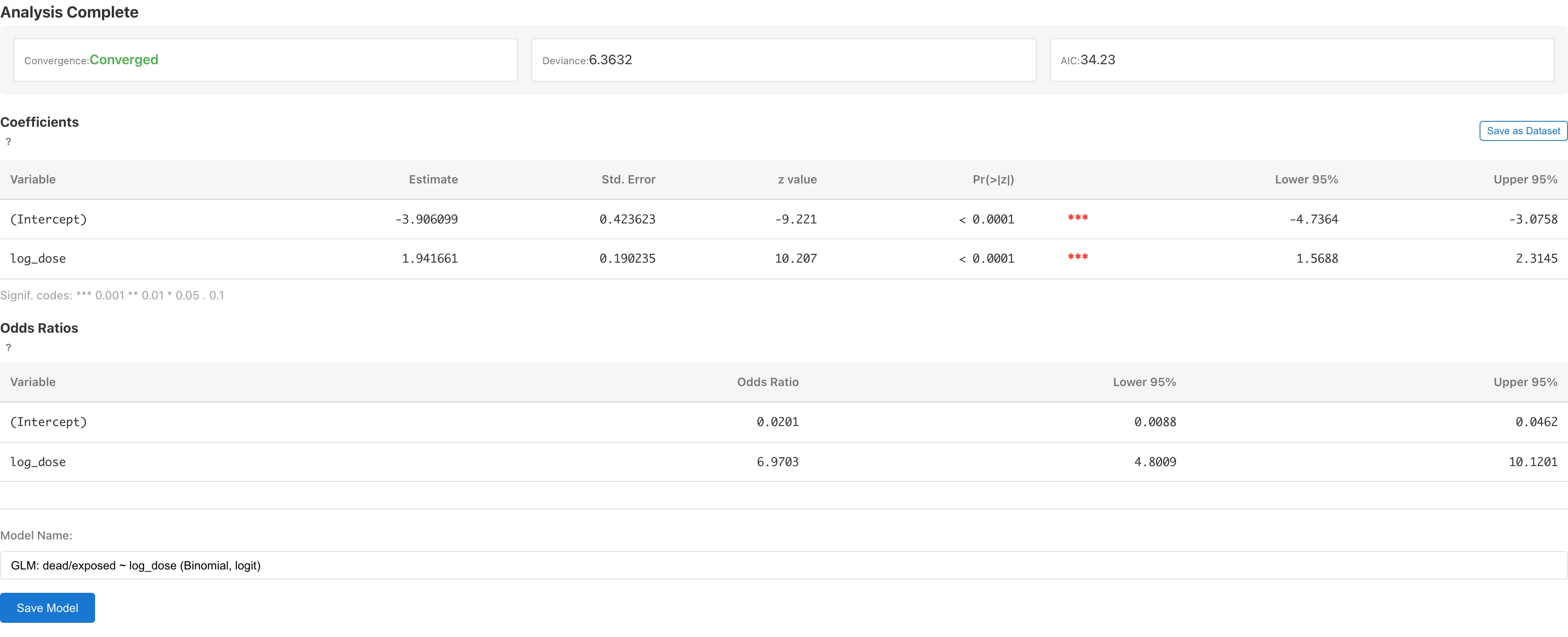
Convergence	Whether the estimation converged. "Converged" indicates normal completion
Deviance	Residual deviance, measuring model fit. Smaller values indicate better fit. Evaluate in conjunction with the residual degrees of freedom ($n - p$, here $8 - 2 = 6$). See the appendix for the mathematical background
AIC	Akaike Information Criterion. Used to compare models — lower values indicate a better balance of fit and complexity. This tutorial builds only one model, but you can create multiple models with different predictors or link functions and compare their AIC values

Read the coefficients table

The Coefficients table has two rows.

(Intercept)

The intercept represents the log-odds $\log(p/(1-p))$ when log_dose = 0 (i.e., dose = 1).

log_dose

The log_dose coefficient is the change in log-odds per unit increase in log_dose (i.e., when dose increases by a factor of $e \approx 2.72$). A positive value means higher concentration increases the probability of death.

The columns in the table:

Column	Meaning
Estimate	The estimated regression coefficient $\hat\beta$, on the log-odds scale (because of the logit link)
Std. Error	Standard error of the estimate
z value	Wald statistic $z = \hat\beta / \text{SE}(\hat\beta)$, asymptotically following the standard normal distribution
Pr(>|z|)	Two-sided p-value testing the null hypothesis that the coefficient is zero
Lower 95% / Upper 95%	95% Wald confidence interval

Interpret coefficients as odds ratios

Logit-link coefficients are on the log-odds scale, which is not intuitive to read directly. Computing $\exp(\hat\beta)$ gives the odds ratio.

For the log_dose coefficient $\hat\beta$, $\exp(\hat\beta)$ is the odds ratio when dose increases by a factor of $e$.

Confidence intervals for the odds ratio are obtained as $\exp(\text{Lower 95\%})$ and $\exp(\text{Upper 95\%})$. If the interval does not include 1, the data suggest that an odds ratio of 1 (no effect) is unlikely. The width of the interval reflects the uncertainty of the estimate — narrower intervals indicate more precise estimation.

To obtain predicted probabilities at specific conditions, save the model and use the prediction feature in the GLM page.

Save the model

Enter a model name in the Model Name field. A default name like "GLM: dead/exposed ~ log_dose (Binomial, logit)" is auto-generated. Click Save Model.

Saving creates a derived dataset that adds diagnostic columns (fitted_values, deviance_residuals, pearson_residuals, leverage, cooks_distance, etc.) to the original data.

After saving, View Diagnostics and View Model Details buttons appear.

Check diagnostic plots

Click View Diagnostics to open the GLM Diagnostics tab.

MIDAS does not show the Normal Q-Q Plot for non-Gaussian GLMs. The normal approximation for deviance residuals holds for grouped binomial data with large trial counts, but is poor for binary data or small trial counts. The plot is therefore disabled for the binomial family as a whole. The remaining three plots:

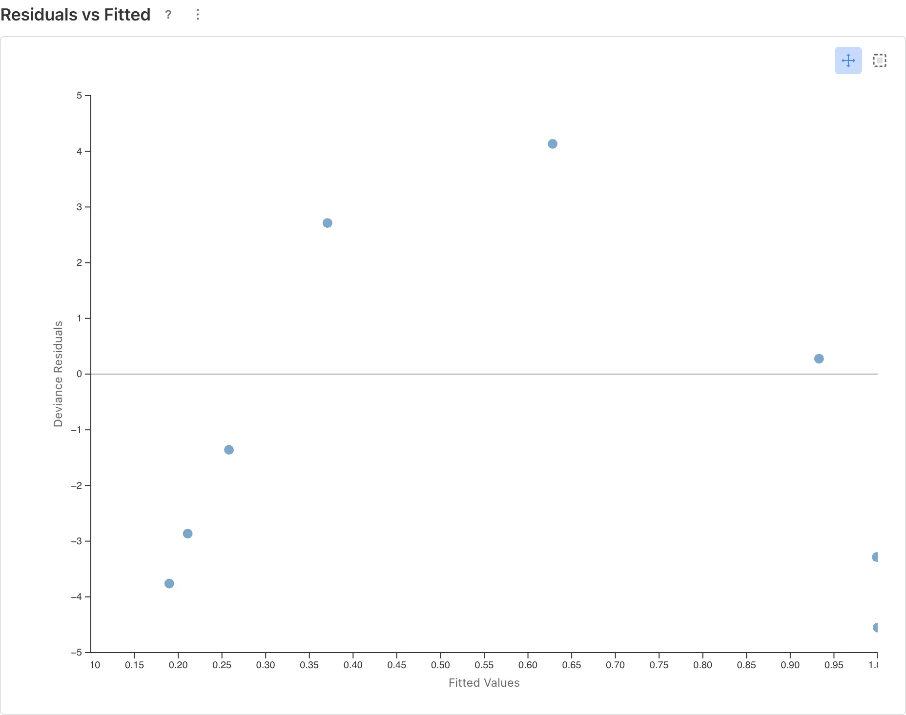
Residuals vs Fitted

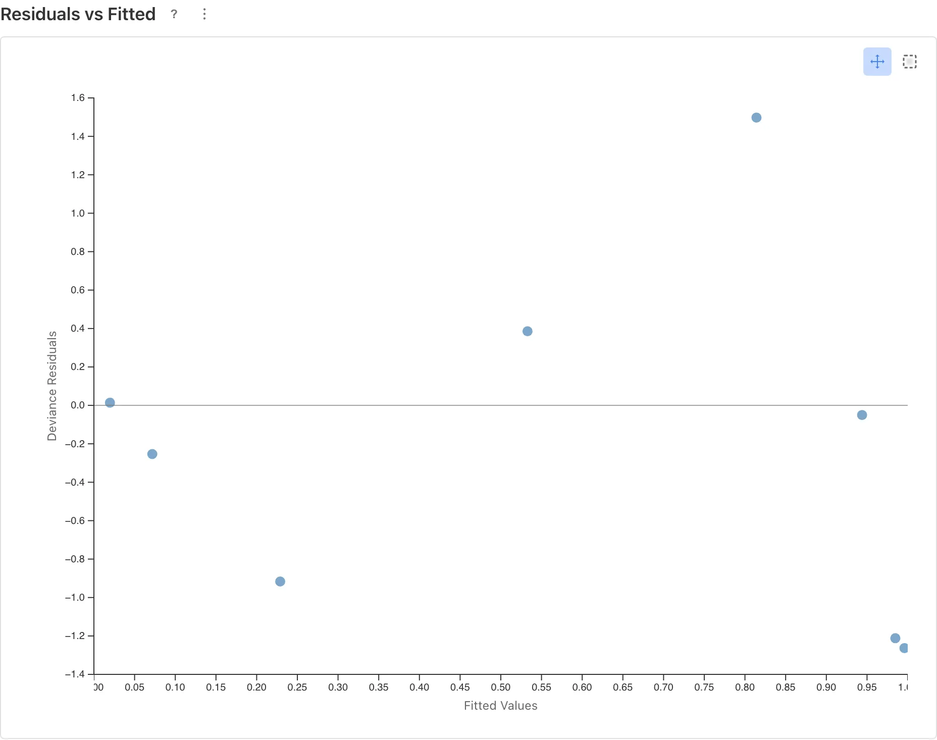
The horizontal axis shows the predicted values (Fitted Values) and the vertical axis shows the residuals (Deviance Residuals). Residuals represent the discrepancy between what the model predicts and the actual data.

Points scattered randomly around the zero line indicate that the model captures the data's trend adequately. With few data points (8 in this example), judging whether a pattern exists is difficult. If no clear pattern is visible, assume no major problem, but subtle departures may go undetected.

A curved pattern (U-shape, inverted U, etc.) means the model's fit is systematically poor in certain ranges of predicted values. GLM assumes a linear relationship between the log-odds and the predictor, so if the actual relationship is not linear, residuals will be biased in specific ranges. This calls for reconsidering the model specification — transforming the predictor or changing the link function.

Scale-Location

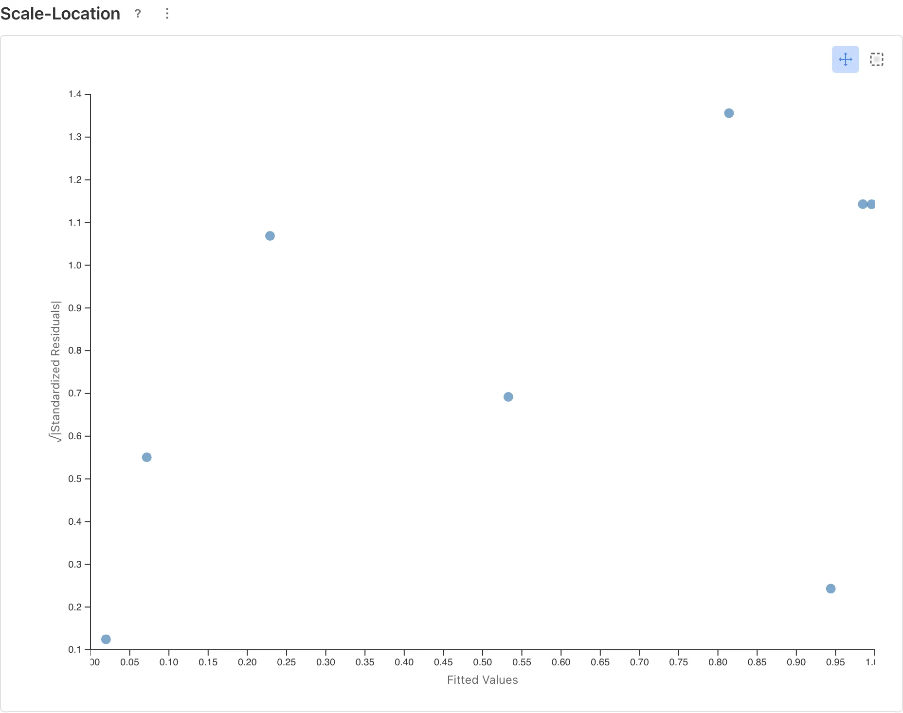
Checks whether the variance structure assumed by the model matches the data. In the binomial family, the variance $np(1-p)$ is inherent to the model, so an upward trend is a sign of overdispersion. See the GLM page for more on overdispersion.

Residuals vs Leverage

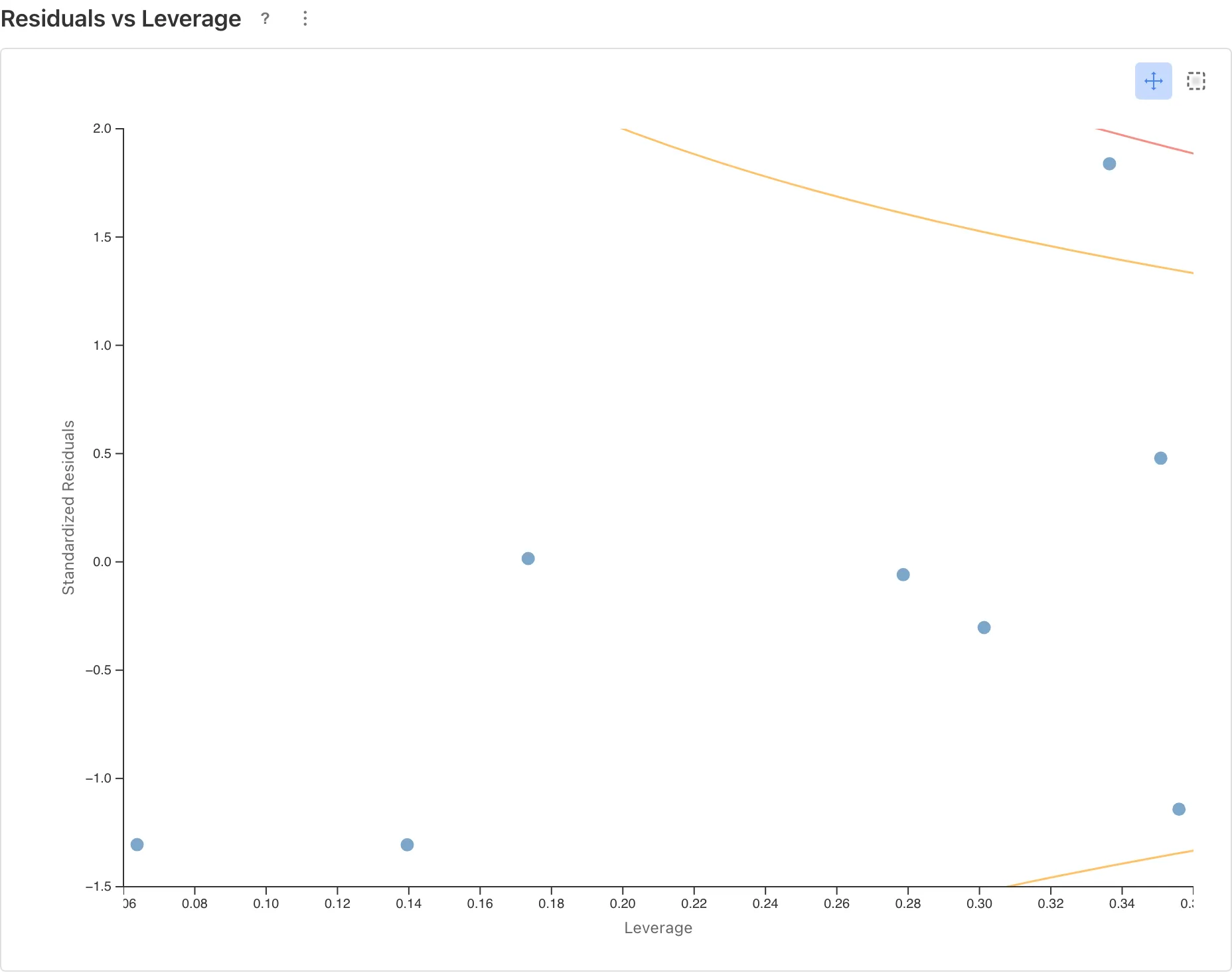
Identifies influential observations. Points outside Cook's Distance contours ($D = 0.5$: orange dashed, $D = 1.0$: red dashed) may substantially change the estimates if removed.

Summarize the results

With the model validated, we can answer the opening question: "how much does mortality increase as concentration rises?"

Relationship between concentration and odds of death

The log_dose coefficient is 1.94. $\exp(1.94) \approx 6.96$, so when concentration increases by a factor of $e \approx 2.72$, the odds of death increase roughly 7-fold.

Since dose doubles at each step, a doubling conversion is practical: $\exp(1.94 \times \log(2)) \approx \exp(1.34) \approx 3.8$. Doubling the concentration multiplies the odds of death by about 3.8.

Estimating the LD50

The LD50 is the concentration at which 50% of insects die. MIDAS does not compute LD50 automatically, so it must be calculated manually from the coefficient table. At 50% mortality the log-odds equals zero, so solving $0 = \hat\beta_0 + \hat\beta_1 \times \log(\text{LD50})$ gives:

$\text{LD50} = \exp\!\left(-\frac{\hat\beta_0}{\hat\beta_1}\right) = \exp\!\left(-\frac{-3.91}{1.94}\right) = \exp(2.01) \approx 7.5 \text{ mg/L}$

This insecticide is estimated to kill half the insects at a concentration of about 7.5 mg/L. Use Save as Dataset from the coefficient table to export the coefficients to the SQL tab.

Interval estimation with the delta method

The value above is a point estimate. Interval estimation requires the covariance of $\hat\beta_0$ and $\hat\beta_1$. Save as Dataset saves both the coefficient table and the variance-covariance matrix as separate datasets. In the SQL tab, you can use the delta method to compute a 95% confidence interval for LD50.

Since $\log(\text{LD50}) = -\hat\beta_0 / \hat\beta_1$, the delta method approximates its variance from a first-order Taylor expansion. The 95% confidence interval is constructed on the log scale and back-transformed via exp, producing an asymmetric interval on the original scale¹.

WITH coef AS (
  SELECT
    MAX(CASE WHEN Variable = '(Intercept)' THEN Estimate END) AS b0,
    MAX(CASE WHEN Variable = 'log_dose'    THEN Estimate END) AS b1
  FROM [GLM Coefficients - bliss1947]
),
cov AS (
  SELECT
    MAX(CASE WHEN row_var = '(Intercept)' AND col_var = '(Intercept)' THEN value END) AS v00,
    MAX(CASE WHEN row_var = '(Intercept)' AND col_var = 'log_dose'    THEN value END) AS c01,
    MAX(CASE WHEN row_var = 'log_dose'    AND col_var = 'log_dose'    THEN value END) AS v11
  FROM [GLM Coefficients - bliss1947 - Covariance]
)
SELECT
  exp(-b0 / b1) AS ld50,
  exp(-b0/b1 - 1.96 * sqrt(
    v00/(b1*b1) + (b0*b0)*v11/(b1*b1*b1*b1) + 2*(-b0)*c01/(b1*b1*b1)
  )) AS lower_95,
  exp(-b0/b1 + 1.96 * sqrt(
    v00/(b1*b1) + (b0*b0)*v11/(b1*b1*b1*b1) + 2*(-b0)*c01/(b1*b1*b1)
  )) AS upper_95
FROM coef, cov

Dataset names depend on the name you entered when saving. The example above uses GLM Coefficients - bliss1947.

What happens with a misspecified model

For comparison, consider using dose as-is without log transformation. The model assumes $\text{logit}(p) = \beta_0 + \beta_1 \times \text{dose}$, but the actual relationship is between log(dose) and log-odds, so this assumption does not match the data.

The Residuals vs Fitted plot reveals the problem.

An inverted U-shape is visible. Residuals are positive at mid-range predicted values (model under-predicts) and negative at both extremes (model over-predicts). This indicates that the relationship between log-odds and dose is not linear.

When this kind of pattern appears in the diagnostic plots, revisit the model specification. Transforming the predictor is one remedy, but changing the link function or adding/removing predictors may also be appropriate.

Review

A summary of what this tutorial covered:

• Data format: Use Binary for individual observations, Grouped for aggregated counts. Data recorded as successes/trials per condition calls for Grouped
• Predictor transformation: Log-transforming dose is standard in dose-response analysis. Use the Add Columns tab to create the transformed column before running GLM
• Coefficient interpretation: Logit-link coefficients are on the log-odds scale. Convert with $\exp(\hat\beta)$ to get odds ratios
• Model validation: Compare deviance to residual degrees of freedom and check diagnostic plots for patterns

For the mathematical background on distribution families and link functions, see GLM Fundamentals.

Appendix

Asymptotic distribution of deviance

In binomial and Poisson GLMs the dispersion parameter $\phi = 1$ is fixed by theory. Under this condition, the residual deviance of a correctly specified model asymptotically follows a $\chi^2(n - p)$ distribution ($n$ = number of observations, $p$ = number of parameters). Dividing deviance by the residual degrees of freedom $n - p$ (i.e., $\hat\phi = D / (n - p)$) therefore yields a value near 1 when the model's assumed variance structure is consistent with the data. A ratio substantially greater than 1 suggests overdispersion.

This $\chi^2$ approximation holds for grouped data where trial counts per group are sufficiently large. For binary data (trial count = 1 per observation), the approximation is poor and deviance/df cannot be used as an overdispersion indicator.

Limitations of Wald confidence intervals

The confidence intervals shown in the coefficients table are Wald intervals ($\hat\beta \pm z_{\alpha/2} \times \text{SE}(\hat\beta)$). Wald intervals are known to have coverage probability below the nominal level (95%) when the sample is small (McCullagh & Nelder, 1989, pp. 118-120). This tutorial's data has only 8 groups, so the confidence interval widths should not be interpreted as highly precise.

References

• Bliss, C. I. (1935). The calculation of the dosage-mortality curve. Annals of Applied Biology, 22(1), 134-167.
• McCullagh, P., & Nelder, J. A. (1989). Generalized Linear Models (2nd ed.). Chapman and Hall/CRC, pp. 108-117.

Footnotes

1. This confidence interval is based on the Wald approximation. With small samples, the actual coverage probability can fall below the nominal level. See Limitations of Wald confidence intervals for details. ↩