Tutorial: Analyzing Successes-and-Trials Data with Logistic Regression
This tutorial estimates how a success probability depends on a condition, using data aggregated as successes and trials per condition. The method is a Grouped Binomial GLM (logistic regression). The example is dose-response data: groups of insects were exposed to an insecticide at increasing concentrations, and the number of deaths was recorded at each concentration.
The same procedure applies to any data with a "K successes out of N trials" structure, regardless of field. Passed units out of inspected units in quality inspection, or cases out of subjects in an epidemiological survey, have the same structure.
This tutorial assumes the basic operations covered in Getting Started.
Load the data
Click Dose Response in the Sample Data section of the launcher screen to load a dataset with 8 rows and 4 columns. You can also open it directly by URL without going through the launcher.
This is synthetic data that the MIDAS project created to mimic an insecticide dose-response experiment. It is not a record of a real experiment.
The license is CC0 1.0. The MIDAS project does not exercise copyright over it, so you can use it freely without attribution.
| Column | Description |
|---|---|
dose | Insecticide concentration (mg/L) |
exposed | Number of insects exposed at that concentration |
dead | Number of those insects that died |
mortality_rate | Mortality rate |
The response used in the analysis is the pair of dead and exposed. mortality_rate is a reference column, dead / exposed rounded to three decimal places, and does not enter the model.
Examine the data structure
In this data, each row represents one concentration condition, not one individual. It mimics an experiment that set eight concentrations doubling from 1.0 to 128.0 mg/L, exposed a separate group of 46 to 52 insects at each concentration, and counted the deaths.
With only 8 rows, the full data fits here.
| dose | exposed | dead | mortality_rate |
|---|---|---|---|
| 1.0 | 50 | 1 | 0.020 |
| 2.0 | 48 | 3 | 0.063 |
| 4.0 | 46 | 8 | 0.174 |
| 8.0 | 50 | 28 | 0.560 |
| 16.0 | 47 | 42 | 0.894 |
| 32.0 | 52 | 49 | 0.942 |
| 64.0 | 49 | 47 | 0.959 |
| 128.0 | 51 | 50 | 0.980 |
Grouped format and Binary format
The Binomial GLM calls this format, with successes and trials aggregated into one row, Grouped, as opposed to Binary, which uses one row per individual. Binary records death = 1 or survival = 0 for each individual, so the 50 insects at 1.0 mg/L become 50 rows. Grouped represents the same 50 records as a single row with dead = 1 deaths and exposed = 50 exposed.
If no predictor varies between individuals, both formats give identical coefficient and standard error estimates1. The only predictor in this data is the concentration, and every individual at the same concentration shares its value, so aggregating loses no information needed for estimation. If you want individual-level predictors such as body weight, you need Binary-format data recorded per individual.
A Grouped row can be treated as a binomial distribution only when the individuals within the row can be regarded as independent and sharing the same death probability. When individuals cluster, as with groups raised in the same container, the actual variability exceeds what the binomial distribution assumes. This excess is called overdispersion, and the diagnostics section checks for signs of it.
Look at the pattern in the data
A scatter plot confirms the relationship expected in dose-response experiments: mortality follows an S-shaped curve against the logarithm of the dose. Open Analysis > Graph Builder..., choose Custom Graph, assign dose to X and mortality_rate to Y, and set the X scale to log in the Scales section. Mortality stays near 0 at low concentrations, approaches 1 at high concentrations, and increases monotonically in between.
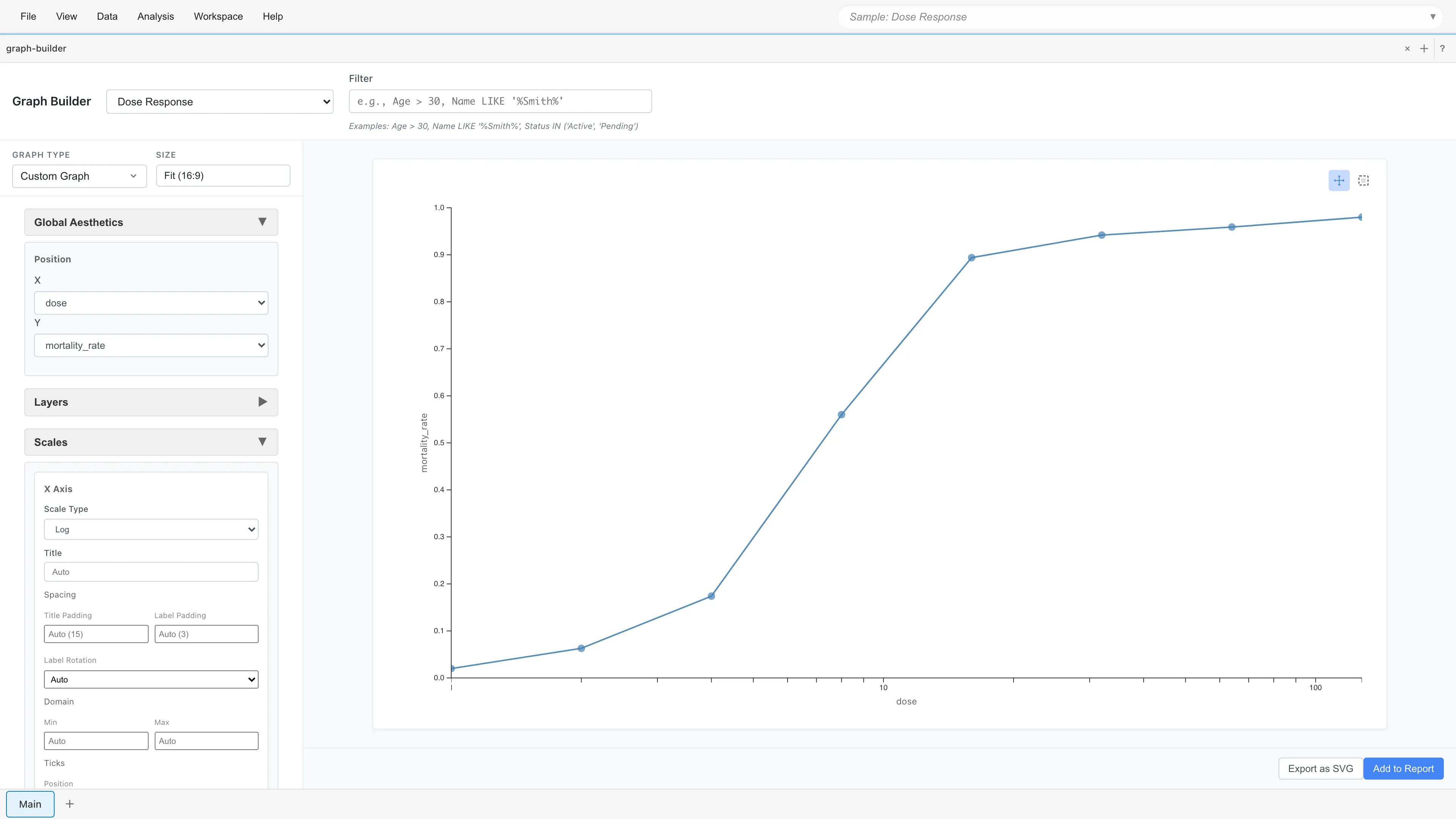
Logistic regression models this S-shape as a linear relationship between the log odds and the predictor. For a death probability , the odds are , and the log odds are their logarithm . Probabilities are confined to the range 0 to 1, but log odds range from to , so the linear expression can represent them directly. This mapping is called the Logit link. See GLM Fundamentals for the mathematics of GLMs, including link functions.
Log-transform the predictor
Following the shape of the scatter plot, use the logarithm of dose as the predictor. The S-shape appeared with a log-scaled axis, so the candidate for a linear relationship with the log odds is log(dose), not dose itself. What happens if you use dose directly is shown in What happens with a misspecified model.
Open Data > Add Columns... and create a derived dataset with a log_dose column. Enter log_dose as the Column name and LN("dose") as the SQL expression. Check the result with Preview, enter a dataset name in Output Name, and click Save as Dataset.
Configure and run the GLM
Open Analysis > Generalized Linear Model (GLM)... and configure the dataset, the distribution family, and the response format and columns.
- Under Dataset, select the derived dataset saved from Add Columns
- Under Distribution Family, select Binomial (Logistic)
- Under Response format, select Grouped (n trials)
- Set Successes to
deadand Trials toexposed
From this specification, MIDAS converts the response to the mortality rate (dead / exposed) and uses exposed as the weight in estimation.
Next, configure the predictor, the link function, and the intercept. Check log_dose under Predictor Variables (X). Leave Link Function at the default Logit and leave Include intercept on.
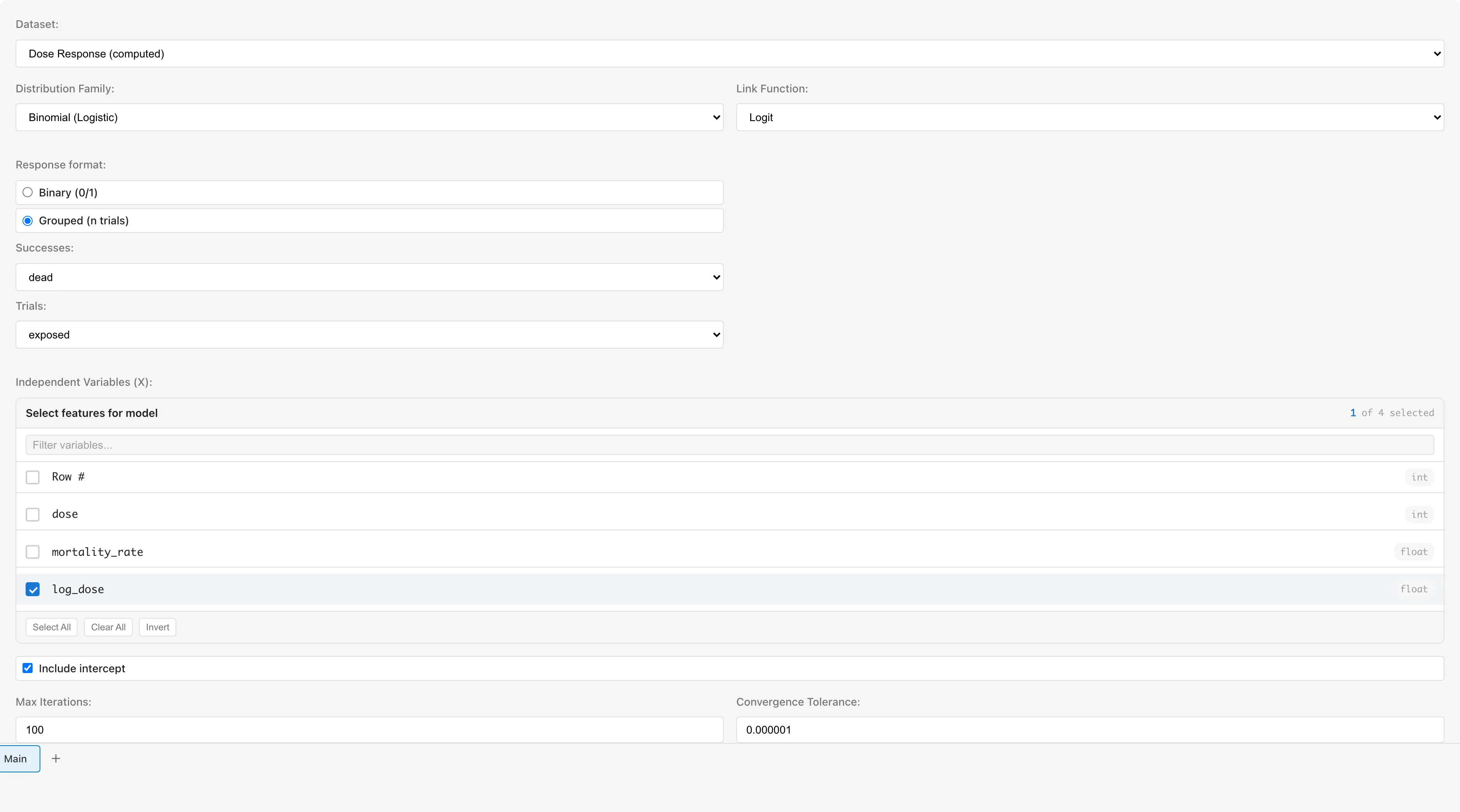
Click Run GLM to start the estimation. The results appear once the estimation converges, and the Convergence History at the end of the results lists the Deviance at each iteration.
Read the results
Check the state of the estimation with Convergence, Residual Deviance, and AIC at the top of the results area. Convergence reads Converged (5 iterations), so the estimation has converged. See The GLM Tab for how to read Residual Deviance and AIC.
Below the fit statistics, Prediction Accuracy Metrics shows the Brier Score, the AUC, and a ROC curve. These metrics are computed on the fitting data itself and are weighted by trials for the successes-and-trials format. See The GLM Tab: In-Sample Prediction Accuracy Metrics for how to read them.
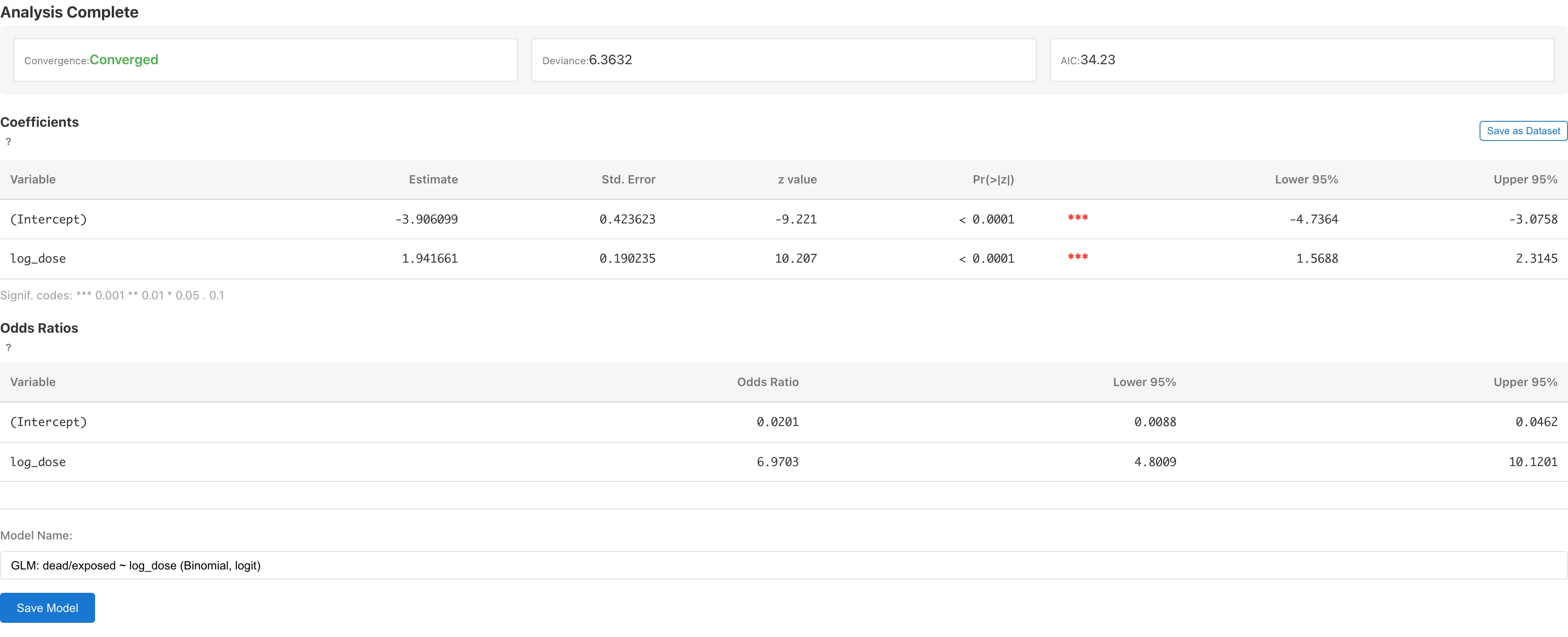
The log_dose row of the coefficients table is the estimate of the relationship between concentration and death probability. The coefficient is the slope on the log-odds scale. It is the change in log odds when log_dose increases by 1, that is, when dose is multiplied by . The estimate, 1.94, is positive, so higher concentrations are estimated to give higher death probabilities.
| Estimate | Std. Error | Lower 95% | Upper 95% | OR | exp(Lower 95%) | exp(Upper 95%) | |
|---|---|---|---|---|---|---|---|
| (Intercept) | -3.906099 | 0.423623 | -4.736386 | -3.075813 | 0.0201 | 0.0088 | 0.0462 |
| log_dose | 1.941661 | 0.190235 | 1.568807 | 2.314515 | 6.9703 | 4.8009 | 10.1200 |
The OR column lets you read the coefficients as odds ratios. OR is the exponentiated Estimate, , and exp(Lower 95%) and exp(Upper 95%) are the 95% confidence interval mapped through the same transformation. The OR for log_dose is 6.97, with a 95% confidence interval from 4.80 to 10.12. When dose is multiplied by , the odds of death are estimated to increase about 7-fold2.
With a design like this one, where the concentration doubles at each step, converting to a per-doubling figure is easier to read. , so each doubling of the concentration is estimated to multiply the odds of death by about 3.8.
Save the model and check the diagnostic plots
Enter a model name under Model Name and click Save Model, and the View Diagnostics button appears. Clicking View Diagnostics opens the GLM Diagnostics tab, which shows the diagnostic plots.
For Binomial models, the checks use three diagnostic plots and the Deviance/df ratio. The GLM Diagnostics tab has four plot panels, but for families other than Gaussian the Normal Q-Q plot is not drawn and its panel shows an explanatory note instead. See The GLM Tab for how to read the Deviance/df ratio.
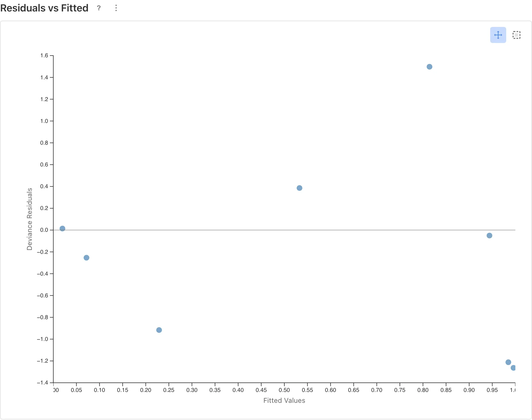
In Residuals vs Fitted, check that the residuals show no systematic pattern. If the points scatter around the horizontal zero line, there is no clear violation of the assumed linear relationship between log odds and predictor. With only 8 points, subtle deviations cannot be detected.
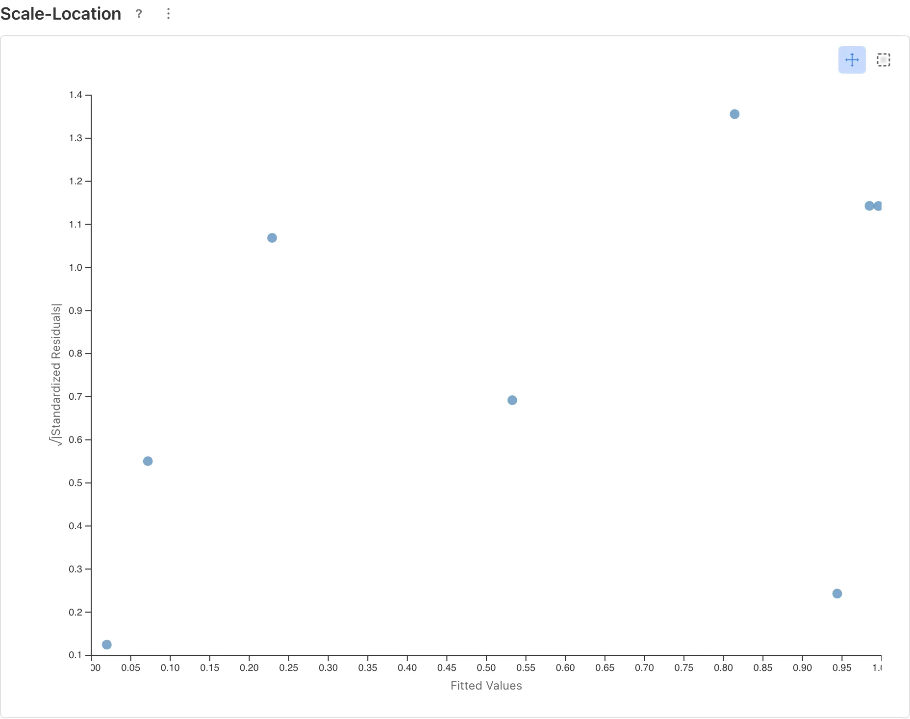
In Scale-Location, check for signs of overdispersion. If the size of the residuals grows with the fitted values, the data may vary more than the model's assumed variance. This plot shows no clear trend, and the Deviance/df ratio, 6.3632 / 6 ≈ 1.06, is close to 1, so there is no sign of overdispersion. See GLM Fundamentals: Variance Functions and Overdispersion for what overdispersion means and how to respond to it.
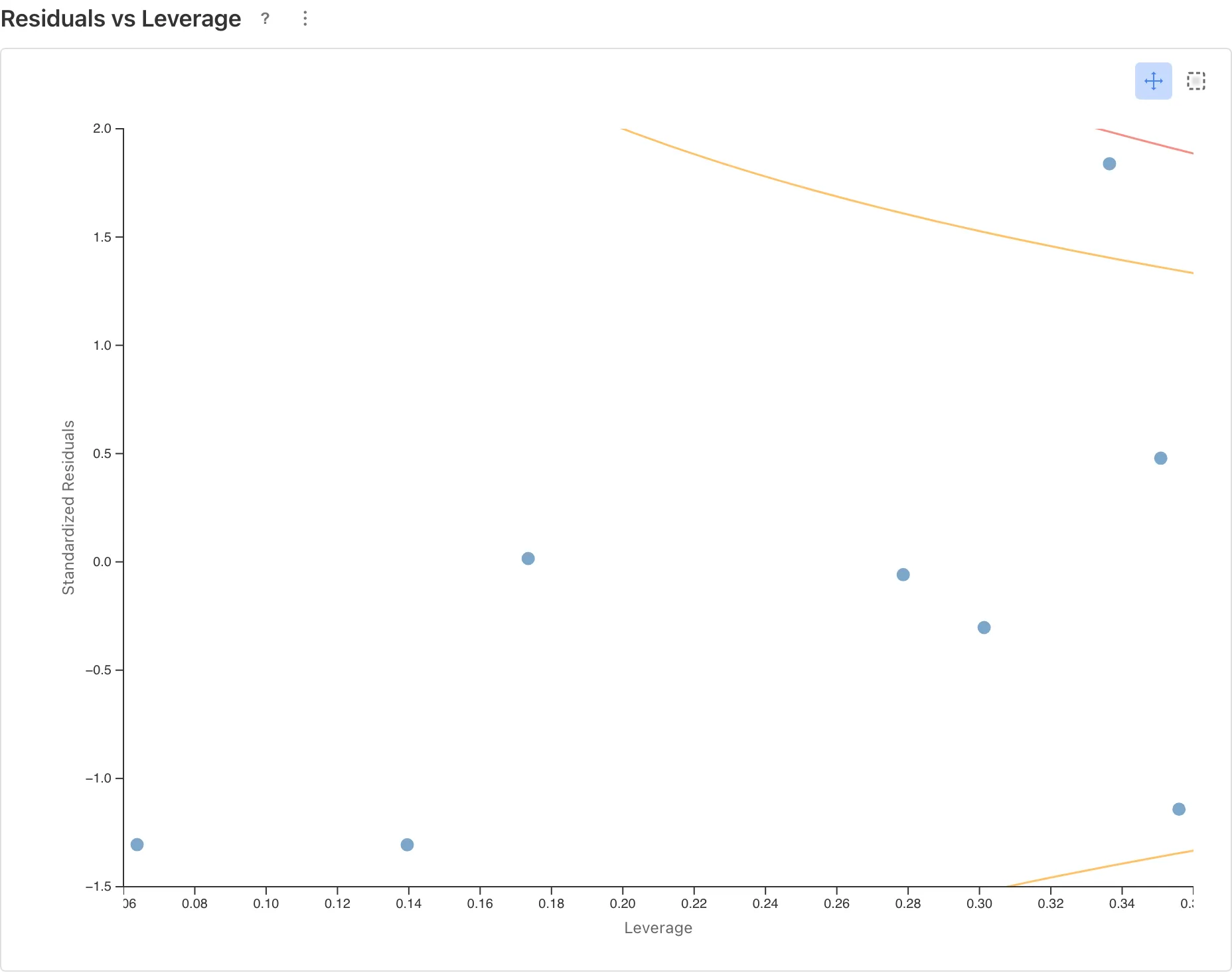
In Residuals vs Leverage, check for observations with outsized influence. The guides are the Cook's Distance contours at D = 0.5 and D = 1.0. A point outside the contours means removing that single row could change the estimates substantially. In this data, the dose = 16 row exceeds the D = 0.5 contour. Its observed mortality is 0.894 against a model prediction of about 0.81, the largest positive deviation. Its Cook's Distance is larger than any other row's, so read the results knowing this row influences the estimates the most.
What happens with a misspecified model
For comparison, fit the model with dose as the predictor without the log transformation. This model assumes a linear relationship between the log odds and dose, but as the scatter plot showed, the relationship in the data is with log(dose). Return to the GLM form, uncheck log_dose under Predictor Variables (X), check dose, and click Run GLM. To see the diagnostic plots, give this model a name too, save it with Save Model, and open View Diagnostics.
The misspecification appears as an inverted-U pattern in Residuals vs Fitted. Residuals lean positive near the middle of the fitted values and negative at both ends. The residuals also grow in magnitude: the deviance residuals, which stayed within 1.5 under the correct specification, now exceed 4.
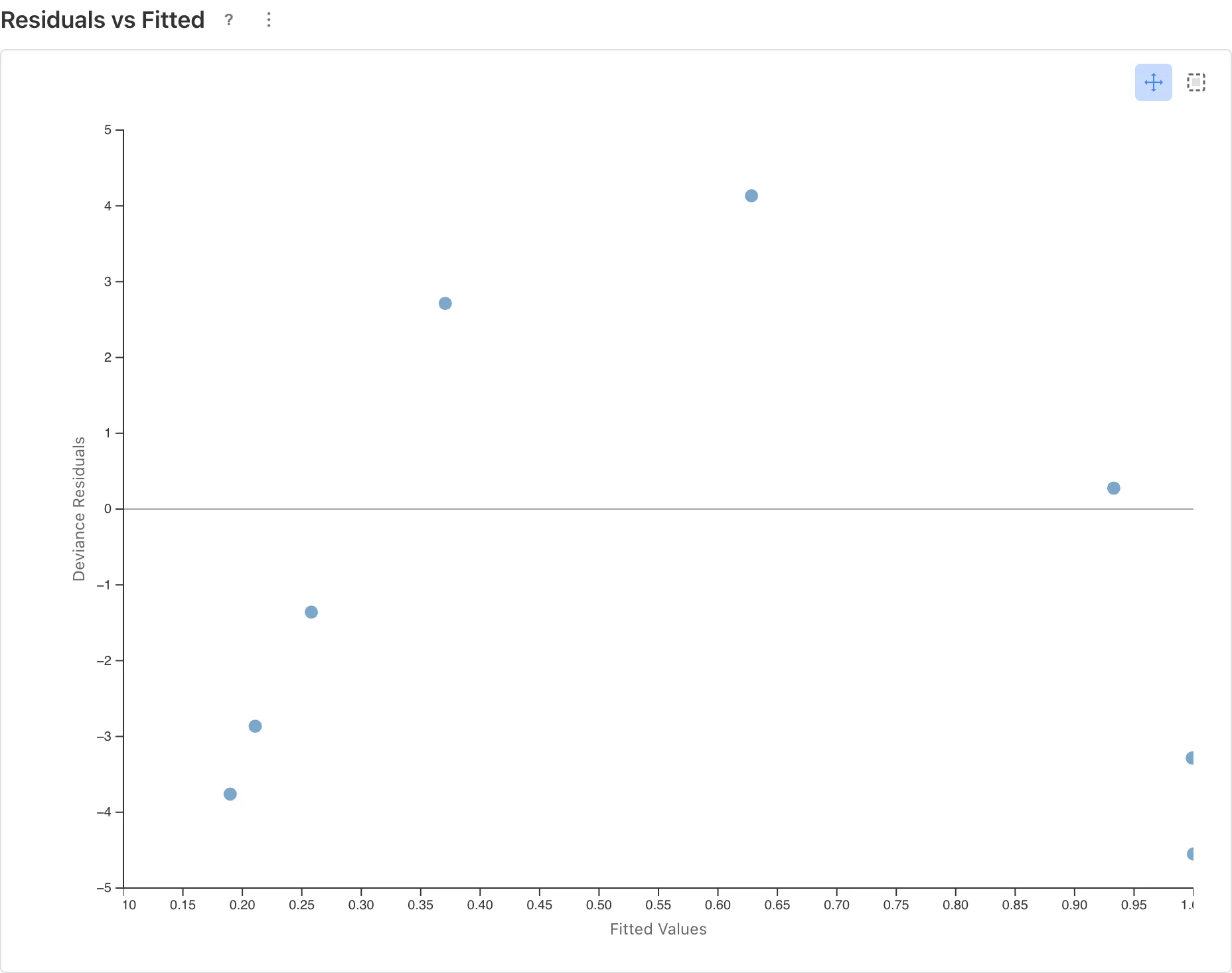
When this kind of pattern appears in the diagnostic plots, revisit the model specification. The candidates are transforming a predictor, changing the link function, and adding predictors.
Compute derived quantities from the coefficients
The concentration at which mortality is exactly 50% can be computed from the coefficients table. Dose-response analysis calls this concentration the LD50. At 50% mortality the log odds are 0, so solving for LD50 gives the following.
Interval estimation for the LD50 uses the coefficient variance-covariance matrix and the delta method. Clicking Save as Dataset on the coefficients table saves the coefficients dataset and, alongside it, the variance-covariance matrix dataset named "{coefficients dataset name} - Covariance". Referencing both in the SQL Query Editor computes the interval; the full SQL is in the appendix. See the glossary for the delta method itself.
Related pages
- The GLM Tab -- Distribution families, link functions, and prediction in detail
- GLM Fundamentals -- The mathematics of link functions, IRLS, and overdispersion
- Sample Datasets -- Contents and license of Dose Response
Appendix
Interval estimation of the LD50 with the delta method
Approximate the variance of with a first-order Taylor expansion, build the confidence interval on the log scale, and map it back with the exponential. Because of the exponential mapping, the interval on the original scale is asymmetric around the point estimate.
If you saved the coefficients dataset under the name "GLM Coefficients", the SQL is as follows. If you saved it under a different name, substitute the two table names in the FROM clauses.
WITH coef AS (
  SELECT
    MAX(CASE WHEN "Variable" = '(Intercept)' THEN "Estimate" END) AS b0,
    MAX(CASE WHEN "Variable" = 'log_dose' THEN "Estimate" END) AS b1
  FROM "GLM Coefficients"
),
cov AS (
  SELECT
    MAX(CASE WHEN row_var = '(Intercept)' AND col_var = '(Intercept)' THEN value END) AS v00,
    MAX(CASE WHEN row_var = '(Intercept)' AND col_var = 'log_dose' THEN value END) AS c01,
    MAX(CASE WHEN row_var = 'log_dose' AND col_var = 'log_dose' THEN value END) AS v11
  FROM "GLM Coefficients - Covariance"
)
SELECT
  exp(-b0 / b1) AS ld50,
  exp(-b0 / b1 - 1.96 * sqrt(v00 / (b1 * b1) + b0 * b0 * v11 / (b1 * b1 * b1 * b1) - 2 * b0 * c01 / (b1 * b1 * b1))) AS lower_95,
  exp(-b0 / b1 + 1.96 * sqrt(v00 / (b1 * b1) + b0 * b0 * v11 / (b1 * b1 * b1 * b1) - 2 * b0 * c01 / (b1 * b1 * b1))) AS upper_95
FROM coef, cov
For this data, the LD50 point estimate is about 7.5 mg/L, with a 95% confidence interval from about 6.3 to 8.9 mg/L.
Footnotes
-
The agreement covers the coefficients and standard errors only. The log-likelihood contains a constant term from the binomial coefficient that differs between formats, so AIC is not comparable across formats. Compare AIC only between models fitted in the same format. ↩
-
This confidence interval is a Wald interval based on the asymptotic normality of the maximum likelihood estimator. Its coverage probability matches the nominal 95% level only in large samples. See GLM Fundamentals: Coefficient Standard Errors and Confidence Intervals for the computation and its properties. ↩
Also available as a Markdown file.