Generalized Linear Mixed Model (GLMM)

The GLMM tab fits random intercept models $g(\mu_i) = x_i'\beta + u_{j[i]}$ , $u_j \sim N(0, \sigma_u^2)$ for data with group structure. It extends GLM by adding random effects. See GLMM Fundamentals for the mathematical background.

For example, when analyzing student test scores from multiple schools, GLMM can estimate the effect of study hours (fixed effect) while accounting for school-level differences (random intercept). When test scores are correlated within schools and study hours vary across schools, ignoring the school differences with GLM leads to underestimated standard errors and confidence intervals that are narrower than they should be.

Basic Usage

Opening GLMM

Select Analysis > Mixed Effects Model (GLMM)... from the menu bar.

Setting Up Variables

GLMM form configuration

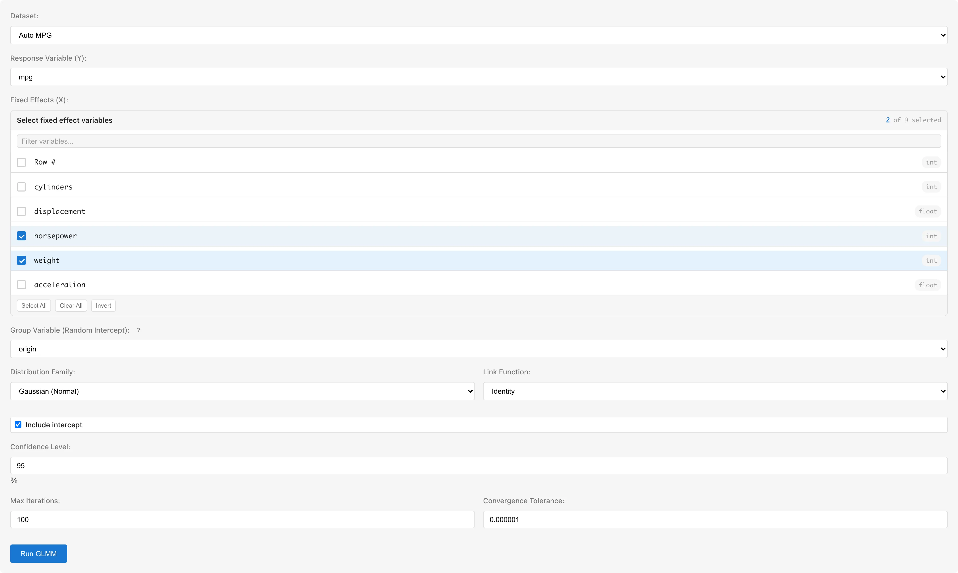
Dataset selects the dataset to analyze.

Response Variable (Y) selects the response variable. Only numeric columns are available.

Fixed Effects (X) selects predictor variables for fixed effects. Only numeric columns are selectable. To use categorical variables, convert them with Dummy Coding first.

Group Variable (Random Intercept) selects the grouping variable for random intercepts. Categorical (nominal/ordinal) or string columns are available.

Distribution Family selects the distribution family:

Family	Default Link	Available Links	Use Case
Gaussian (Normal)	Identity	Identity, Log	Continuous values
Binomial (Logistic)	Logit	Logit, Probit	Binary data
Poisson (Count)	Log	Log, Identity	Count data
Gamma	Inverse	Inverse, Log, Identity	Positive continuous

Link Function selects the link function. Defaults to the canonical link for the selected family. Available options depend on the selected family (see table above).

Link Function	Formula	Description
Identity	$\eta = \mu$	No transformation. Canonical link for Gaussian
Logit	$\eta = \log\!\bigl(\mu / (1 - \mu)\bigr)$	Log-odds transformation. Canonical link for Binomial
Log	$\eta = \log(\mu)$	Log transformation. Canonical link for Poisson. Ensures $\mu > 0$
Inverse	$\eta = 1/\mu$	Reciprocal transformation. Canonical link for Gamma
Probit	$\eta = \Phi^{-1}(\mu)$	Inverse CDF of the standard normal distribution. Corresponds to a latent normal variable model

See GLM: Link Functions for the mathematical properties of canonical links.

Include intercept toggles the intercept term (default: on).

Confidence Level sets the confidence level for confidence intervals (default: 95%, range: 50--99.99%). This is reflected in the Lower N% / Upper N% columns of the Fixed Effects table. The Model Detail tab opened after saving has the same input pre-filled with the saved value, and you can change it there to recompute the CI without modifying the saved value.

Advanced Options

Max Iterations: Maximum optimization iterations (default: 100)
Convergence Tolerance: Convergence threshold (default: 1e-6)

Running the Analysis

Click Run GLMM. The estimation algorithm differs by family (see details). While the analysis runs, a progress bar and the estimation stage appear below the form.

Understanding Results

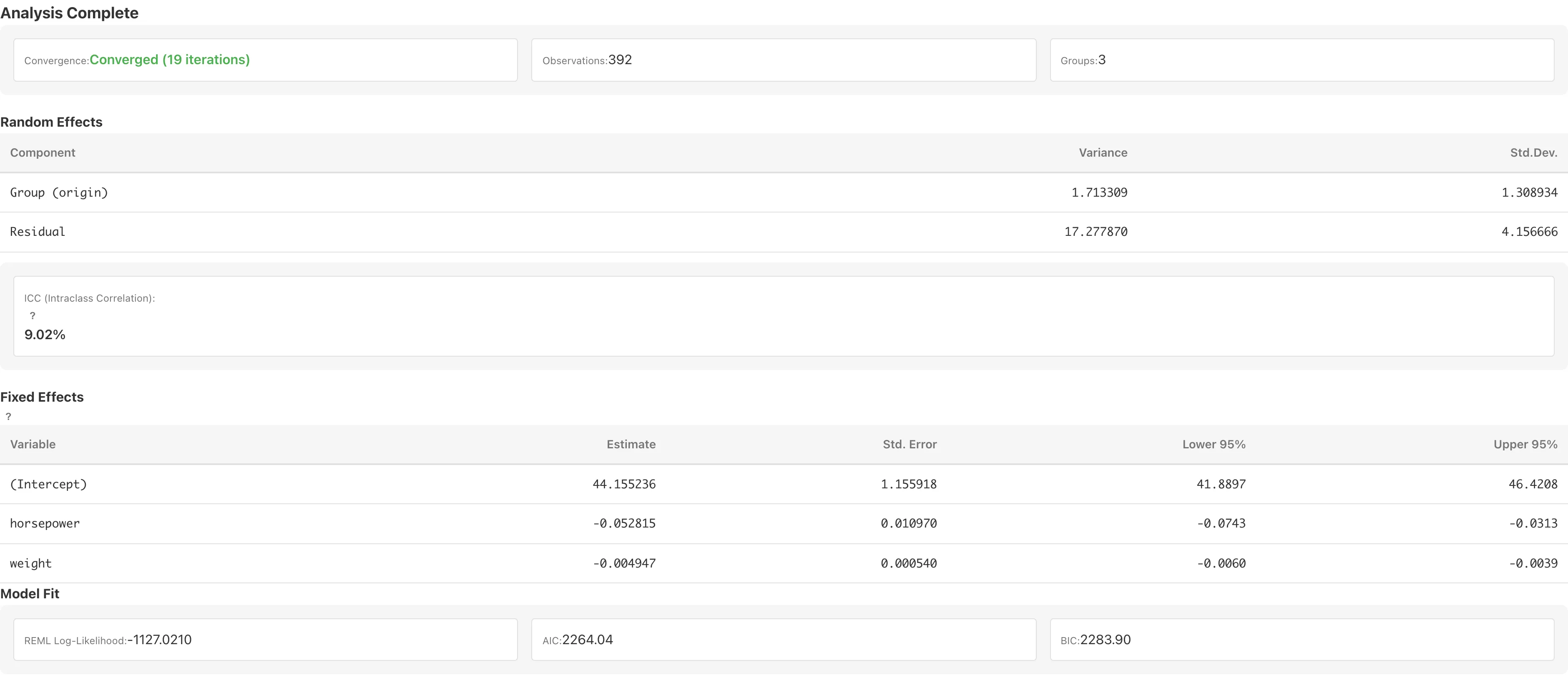
GLMM analysis results (Random Effects, ICC, Fixed Effects, Model Fit)

Random Effects

Displays variance components for random effects.

Column	Description
Component	Name of the variance component. `Group (variable name)` for the group variable variance, `Residual` for residual variance
Variance	Variance estimate: $\sigma_u^2$ for the group variable, $\sigma_e^2$ for the residual
Std.Dev.	Square root of the variance

For Poisson and Binomial families, the Residual row is not shown because the dispersion parameter is fixed at $\phi = 1$ .

The residual variance $\sigma_e^2$ is a property of the distribution family (Gaussian: $\operatorname{Var}(Y \mid \mu) = \sigma_e^2$ ; Gamma: $\operatorname{Var}(Y \mid \mu) = \sigma_e^2 \mu^2$ ) and does not depend on the link function. The link function determines how fitted values $\hat\mu = g^{-1}(\eta)$ are computed from the linear predictor, which in turn affects diagnostic residuals (deviance and Pearson) through family-specific formulas.

ICC (Intraclass Correlation Coefficient)

ICC represents the share of unexplained variance attributable to between-group differences ( $\text{ICC} = \sigma_u^2 / (\sigma_u^2 + \sigma_e^2)$ ). MIDAS computes ICC only for the following family+link combinations, where $\sigma_e^2$ has a theoretical basis:

Family	Link	$\sigma_e^2$
Gaussian	identity	REML estimate
Binomial	logit	$\pi^2/3$ (threshold model)
Binomial	probit	$1$ (threshold model)

For all other combinations — Poisson (all links), Gamma (all links), and Gaussian with the log link — no theoretically grounded residual variance exists, so N/A (ICC not defined) is shown instead of an ICC value. See GLMM Fundamentals for details.

The interpretation of ICC depends on the nature of the data and the research objective. Group size should also be considered (see When to Use GLMM vs GLM). For Binomial models, ICC is computed on the latent (link) scale, not the probability scale (see GLMM Fundamentals).

Fixed Effects

Coefficient table for fixed effects.

Column	Description
Variable	Variable name
Estimate	Regression coefficient $\hat\beta$
Std. Error	Standard error. For Gaussian + identity, computed via $(X'V^{-1}X)^{-1}$ using the Woodbury formula. For all other combinations, an approximation based on the working weight matrix at PIRLS convergence
Lower N% / Upper N%	Wald-based confidence interval $\hat\beta \pm z_{1-\alpha/2} \times \text{SE}(\hat\beta)$ , where N is the selected confidence level. MIDAS always uses the standard normal distribution for GLMM fixed effects

When the link function is logit or log, the following columns are added:

Column	Description
OR / IRR / exp(Est.)	Exponentiated estimate $\exp(\hat\beta)$ . Displayed as odds ratio (OR) for logit link, incidence rate ratio (IRR) for log link with Poisson, and exp(Est.) for log link with other families
exp(Lower N%) / exp(Upper N%)	Exponentiated confidence interval bounds

Coefficient interpretation follows GLM conventions (on the link function scale). See GLM coefficient interpretation for details.

The confidence intervals are based on a normal approximation, which can be too narrow when the number of groups is small. See GLMM Fundamentals: Fixed Effect Inference for details.

Model Fit

Metric	Description
REML Log-Likelihood / Log-Likelihood (Laplace)	Log-likelihood (Gaussian + identity: REML, all other combinations: Laplace approximation)

For Gaussian + identity, the REML log-likelihood including the constant term $-\frac{n-p}{2}\log(2\pi)$ ( $n$ : number of observations, $p$ : number of fixed-effect parameters including the intercept) is displayed. For all other combinations, the Laplace-approximated marginal log-likelihood is displayed.

AIC ( $-2\ell + 2k$ ) and BIC ( $-2\ell + k\log n$ ) are also displayed, where $k$ is the total number of fixed-effect parameters and variance components. When using AIC/BIC for mixed models, note the limitations described in GLMM Fundamentals: AIC/BIC Limitations. REML-based AIC (Gaussian + identity) can only compare models with identical fixed-effect structure. For Laplace-approximated log-likelihoods (all other combinations), the approximation error propagates into any information criterion derived from it. Models with different families or links cannot be compared by AIC, BIC, or log-likelihood, because the log-likelihood basis (REML vs. Laplace) and scale differ.

BLUP (Random Effect Predictions)

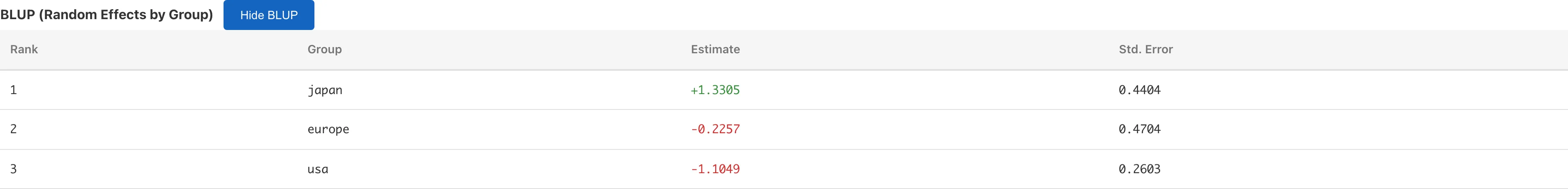
BLUP table showing random effect predictions by group

Displays the predicted random intercept (BLUP) for each group.

Column	Description
Group	Group variable value
Random Intercept	Predicted random intercept. Smaller groups are shrunk more toward the overall mean (0) (shrinkage details)
Std. Error	Standard error of the prediction. The square root of the conditional variance; larger for smaller groups
Rank	Rank of Random Intercept in descending order

For all combinations other than Gaussian + identity, random effects are estimated as conditional modes of the posterior distribution. They exhibit shrinkage similar to the Gaussian + identity BLUP but are not strictly BLUPs. In that case the Std. Error is a posterior-based standard error and may not be directly usable for constructing prediction intervals.

Saving and Diagnostics

Enter a model name in Model Name and click Save Model to save the model to the project. A diagnostic derived dataset is automatically created on save.

Column	Description
`fitted_values`	Predicted values (fixed + random effects)
`deviance_residuals`	Deviance residuals
`pearson_residuals`	Pearson residuals
`group_random_effect`	Group random intercept (BLUP)

For Gaussian + identity, the deviance and Pearson residuals both equal the raw residual $y_i - \hat y_i$ , so deviance_residuals and pearson_residuals hold the same values.

After saving, View Model Details and View Diagnostics buttons become available. Model Detail displays the fixed effects coefficient table and a BLUP table (per-group random intercept estimates). The BLUP table shows up to 50 rows by default; when there are more groups, click Show all N rows (N is the total number of groups) to expand the full list. Use the Add to Report button to add both the coefficients table and the BLUP table to a report.

Notes

Current Limitations

The current GLMM implementation supports random intercept models ( $(1 \mid \text{Group})$ ) only. Random slopes ( $(x \mid \text{Group})$ ) and crossed random effects are not supported.

The GLM tab offers the Negative Binomial family, but GLMM does not.

When to Use GLMM vs GLM

When ICC is small, ignoring group structure and using GLM produces nearly identical results. The impact depends not only on ICC but also on group size; the design effect $\text{DEFF} = 1 + (\bar n - 1) \times \text{ICC}$ provides a rough guide (see GLMM Fundamentals). When ICC is large, GLM violates the independence assumption between observations, leading to underestimated standard errors. GLMM explicitly models within-group correlation, enabling valid inference.

Automatic Exclusion of Missing Values

Rows containing missing values, non-numeric values, or infinity are automatically excluded. The Observations value in the results is the number of observations after exclusion. This is listwise deletion. See Missing Data Mechanisms for conditions under which it yields valid estimates.

Convergence Issues

If the model fails to converge:

Increase Max Iterations (100 → 500)
Relax Convergence Tolerance (1e-6 → 1e-4)
Very few groups (2-3) can make variance component estimation unstable
Large scale differences between predictors may cause the GLM initial-value estimation to fail (internal scaling is applied, but extreme cases may still have issues)

Singular Fit

A "Singular fit" warning appears when the random effect variance estimate is at or near zero — the estimate has reached the boundary of the parameter space. Possible causes:

The grouping variable explains very little variation in the response
The sample size or number of groups is too small to separate group-level variation from residual variation

When singular fit occurs, ICC and variance component estimates should be interpreted with caution. A fixed-effects-only model (GLM) may be more appropriate.