Survival Analysis

MIDAS provides two survival analysis methods:

Kaplan-Meier: Estimate survival curves and compare groups (RMST). Visually assess differences in survival between groups and quantify them using restricted mean survival time
Cox Regression: Estimate the effect of covariates on hazard. Evaluate the simultaneous impact of multiple variables on survival time

See Survival Analysis Fundamentals for the mathematical background.

Data Requirements

Survival analysis requires two variables:

Time variable: Time to event (numeric)
Event variable: Indicates whether the event occurred. The following formats are supported:
- int64: 1 = event, 0 = censored
- Boolean: true = event, false = censored

float64 columns cannot be selected as the event variable. If a column stores 0/1 values as decimals, convert it to int64 with Column Type Conversion.

See Survival Analysis Fundamentals for how censoring is handled. MIDAS only supports right censoring. Left censoring, interval censoring, and competing risks are not supported.

Kaplan-Meier

The Kaplan-Meier method is a nonparametric estimator of the survival function (formulation).

Basic Usage

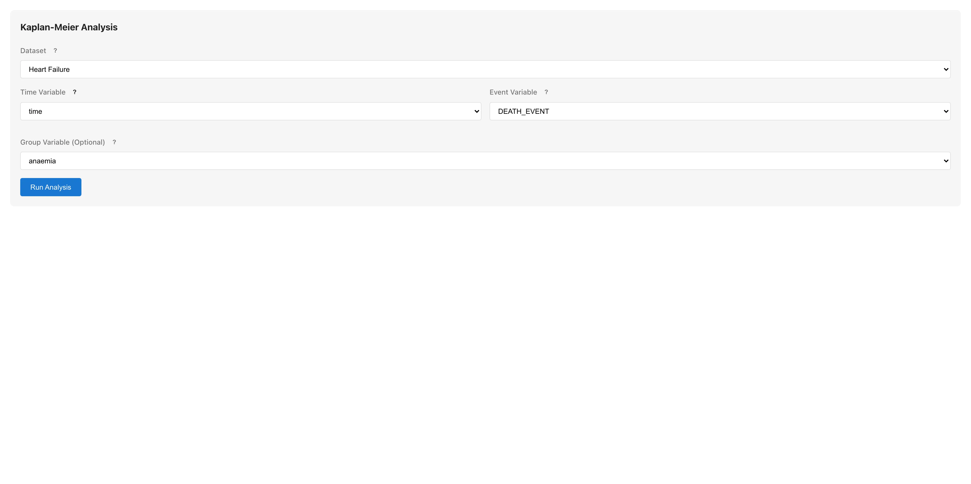
Select Analysis > Survival Analysis > Kaplan-Meier... from the menu bar
Select the Time Variable
Select the Event Variable
Optionally select a Group Variable for group comparison
Click Run Analysis

Kaplan-Meier form configuration

Understanding Results

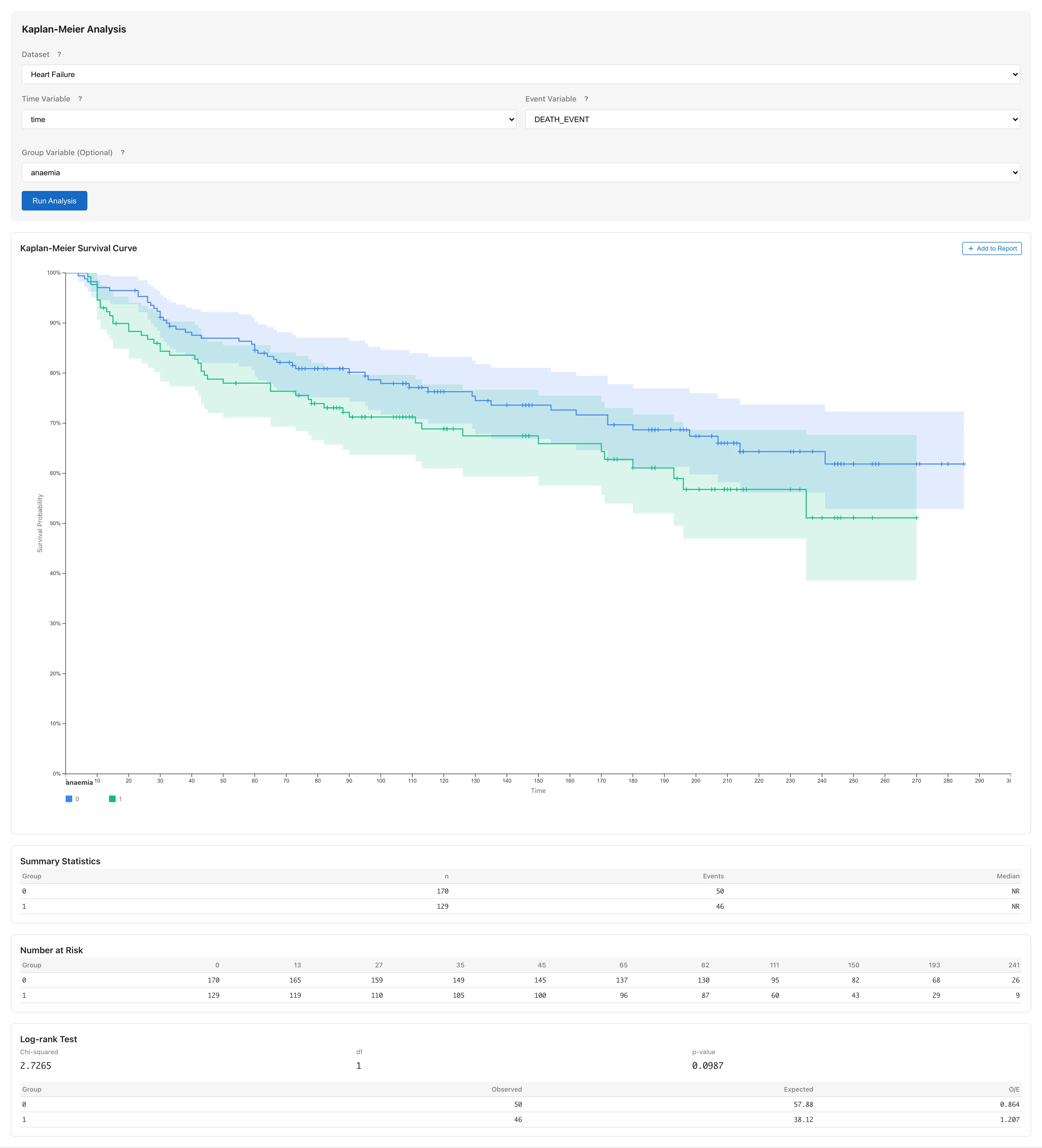
Group comparison results (survival curves, Summary Statistics, Number at Risk, RMST)

Survival Curve

Plots survival probability $S(t)$ against time. Displayed as a step function that decreases at each event time. Censoring times are marked with a + symbol on the curve. A + mark on a flat segment indicates that subjects were lost to follow-up during that interval. A pointwise confidence band (95% by default) is shown. A pointwise band consists of individual intervals at each time point and does not guarantee simultaneous coverage of the entire curve, computed using the log transformation method (details).

Adjust the confidence level with the Confidence Level input.

Summary Statistics

Column	Description
Group	Group name (when Group Variable is specified)
n	Number of observations
Events	Number of events
Median	Median survival time, the earliest time when $S(t) \leq 0.5$ . Displayed as NR (Not Reached) if not reached within the observation period
nn% CI	Confidence interval for the median, obtained by inverting the pointwise confidence band of the survival function. A bound is displayed as NR when the corresponding survival CI bound does not cross $0.5$

Number at Risk

Shows the risk set size (the number of subjects who have not yet experienced the event and have not been censored) at each time point.

RMST (Restricted Mean Survival Time)

The average survival time estimated as the area under the Kaplan-Meier curve from 0 to a restriction time $\tau$ (formulation). Per-group RMST with SE and confidence interval is displayed.

Column	Description
Group	Group name
RMST	Restricted mean survival time estimate
SE	Standard error (Greenwood variance-based)
nn% CI	Confidence interval for RMST (Wald-type)

Restriction Time $\tau$

RMST is the area under the KM curve up to $\tau$ , so the choice of $\tau$ affects the result. The default is the upper bound of the range commonly observed across all groups (the smallest of each group's maximum observed time). Change it with the RMST Restriction Time input. In the interval after the last observed event, the integration assumes the KM curve stays at its last value (this also happens within the maximum observed time when only censoring follows the last event). The longer this interval, the more the uncertainty of RMST may be underestimated.

Group Differences

When a Group Variable is specified and there are two or more groups, pairwise RMST differences and their confidence intervals are displayed. For three or more groups, the per-pair confidence intervals are unadjusted for multiplicity.

Notes

Rows with missing values in the time or event variable are automatically excluded (listwise deletion; see Missing Data Mechanisms for validity conditions). When rows are excluded, the results show the number of excluded rows as "N rows excluded due to missing values."

Adding to Reports

Click Add to Report to add the survival curve to a report.

Cox Regression

The Cox proportional hazards model is a semiparametric model that estimates the effect of covariates on hazard (formulation and theory).

Basic Usage

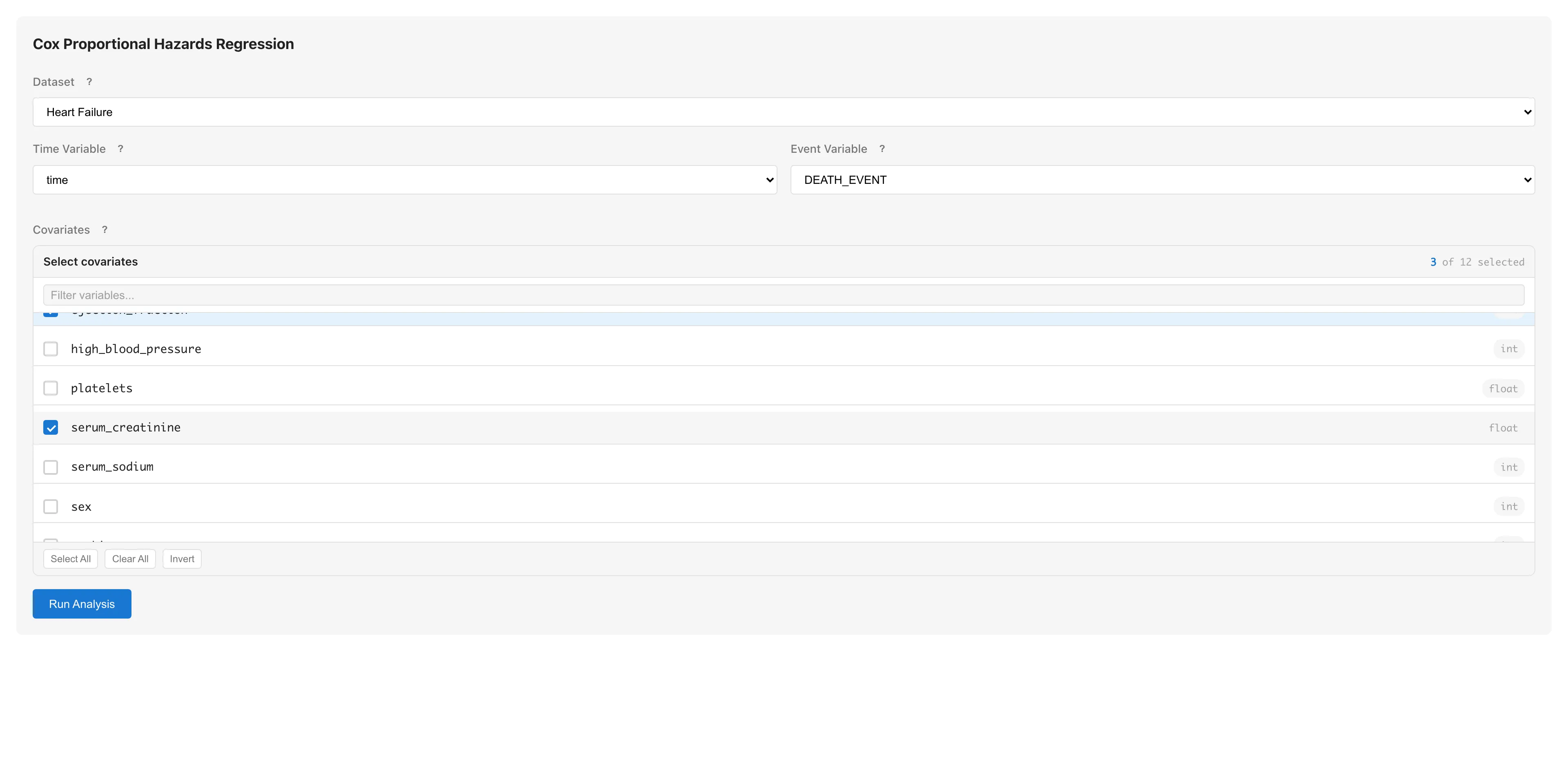
Select Analysis > Survival Analysis > Cox Regression... from the menu bar
Select the Time Variable
Select the Event Variable
Select one or more Covariates (numeric with interval or ratio scale, or boolean)
Click Run Analysis

Columns whose scale is set to nominal or ordinal, as well as date/datetime columns, are grayed out in the list and cannot be selected. To use categorical variables with three or more levels as covariates, convert them with Dummy Coding first (boolean variables can be selected directly).

Cox regression form configuration

Understanding Results

Cox Proportional Hazards Regression

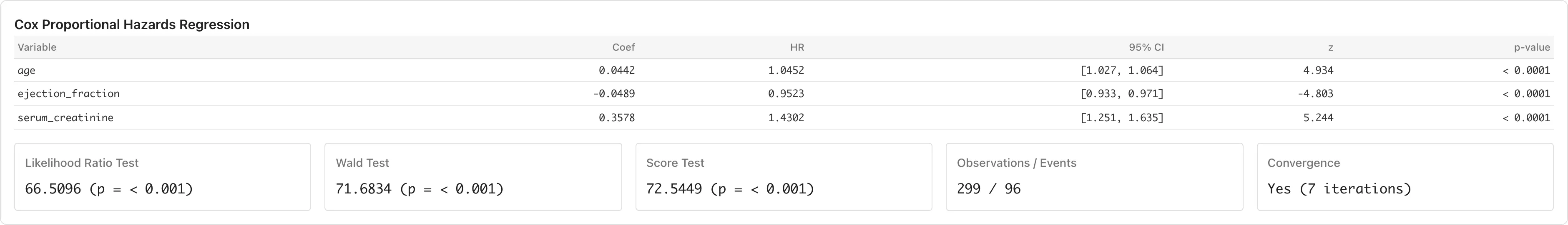
Cox Proportional Hazards Regression section

The upper coefficients table shows the following columns for each covariate.

Column	Description
Variable	Variable name
Coef	Regression coefficient $\beta$
SE	Standard error
HR	Hazard ratio $\exp(\beta)$
CI	Confidence interval for the hazard ratio. The column header reflects the selected confidence level (e.g., "95% CI")

A hazard ratio greater than 1 indicates that an increase in the covariate raises the hazard; less than 1 indicates it lowers the hazard. See Survival Analysis Fundamentals for detailed interpretation.

Below the table, model fit metrics are reported.

Metric	Description
Concordance Index	Harrell's C statistic. The proportion of comparable pairs where the risk score ordering agrees with the event ordering. 0.5 means no discrimination, 1.0 means perfect discrimination. The standard error in parentheses is based on the influence function
AIC	Akaike Information Criterion ( $-2\ell + 2p$ ), where $\ell$ is the partial log-likelihood and $p$ is the number of coefficients. Used for model comparison
Log Partial Likelihood	Partial log-likelihood $\ell(\hat\beta)$ , the basis for AIC

Adjusted Survival Curve

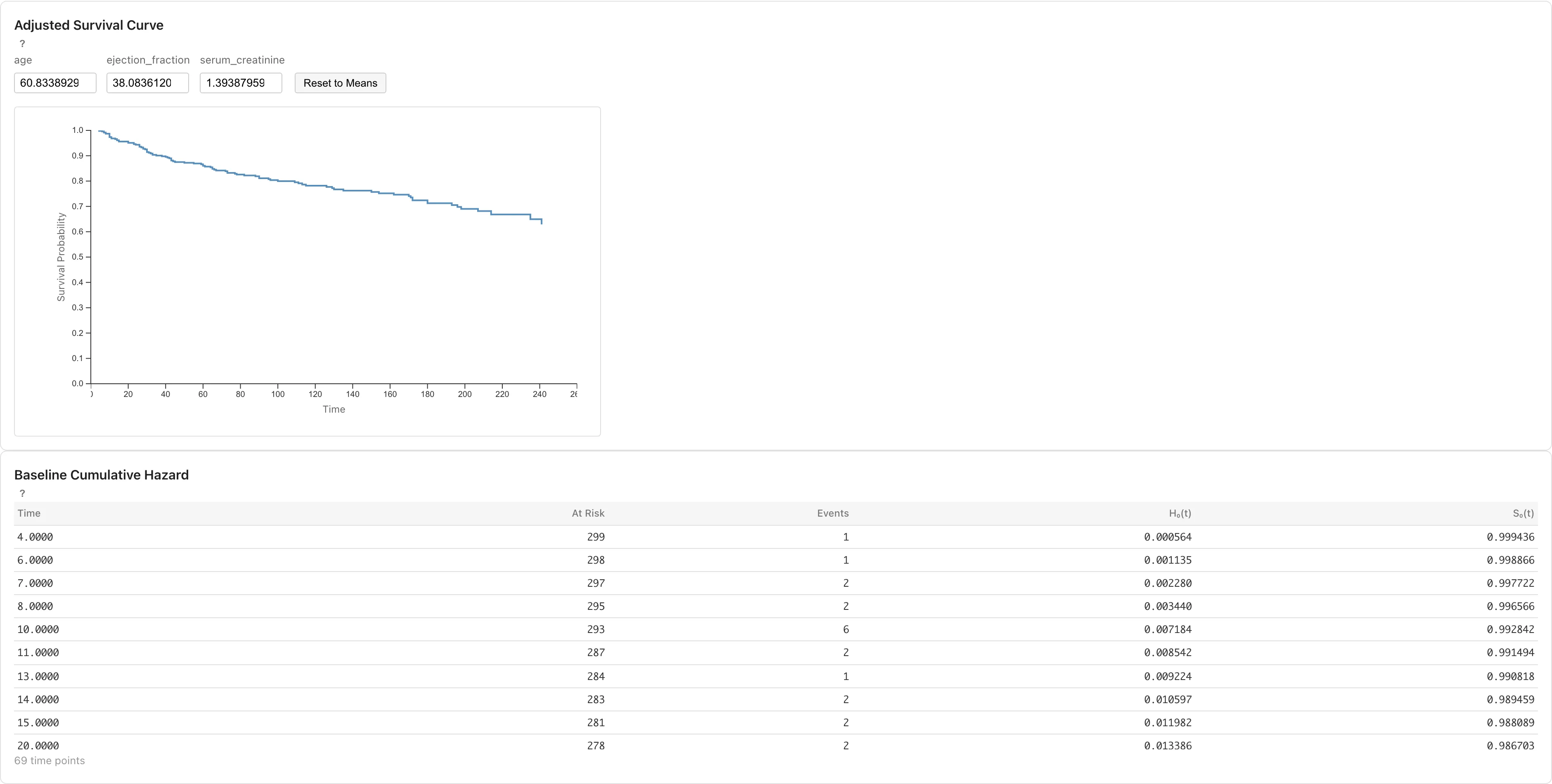
Adjusted survival curve and baseline cumulative hazard table

The adjusted survival curve plots predicted survival probability $S(t|X)$ for a specific set of covariate values $X$ . It is computed from the baseline cumulative hazard and the estimated coefficients (formulation).

Each covariate has an input field, defaulting to the sample mean. Changing a value updates the curve immediately, so you can compare predicted survival across different covariate profiles. Reset to Means restores the defaults.

Baseline Cumulative Hazard

Below the adjusted survival curve, the baseline cumulative hazard table lists the following values at each event time point.

Column	Description
Time	Event time
At Risk	Number of subjects in the risk set
Events	Number of events at this time
H₀(t)	Cumulative baseline hazard
S₀(t)	Baseline survival function $\exp(-H_0(t))$

The baseline corresponds to all covariates set to zero. When zero is not a realistic value given the variable scales, use the adjusted survival curve with realistic covariate values (such as the sample mean) to inspect $S(t|X)$ .

Proportional Hazards Diagnostics

Proportional hazards diagnostics (correlation table, Schoenfeld residual plots, Log-Log plot)

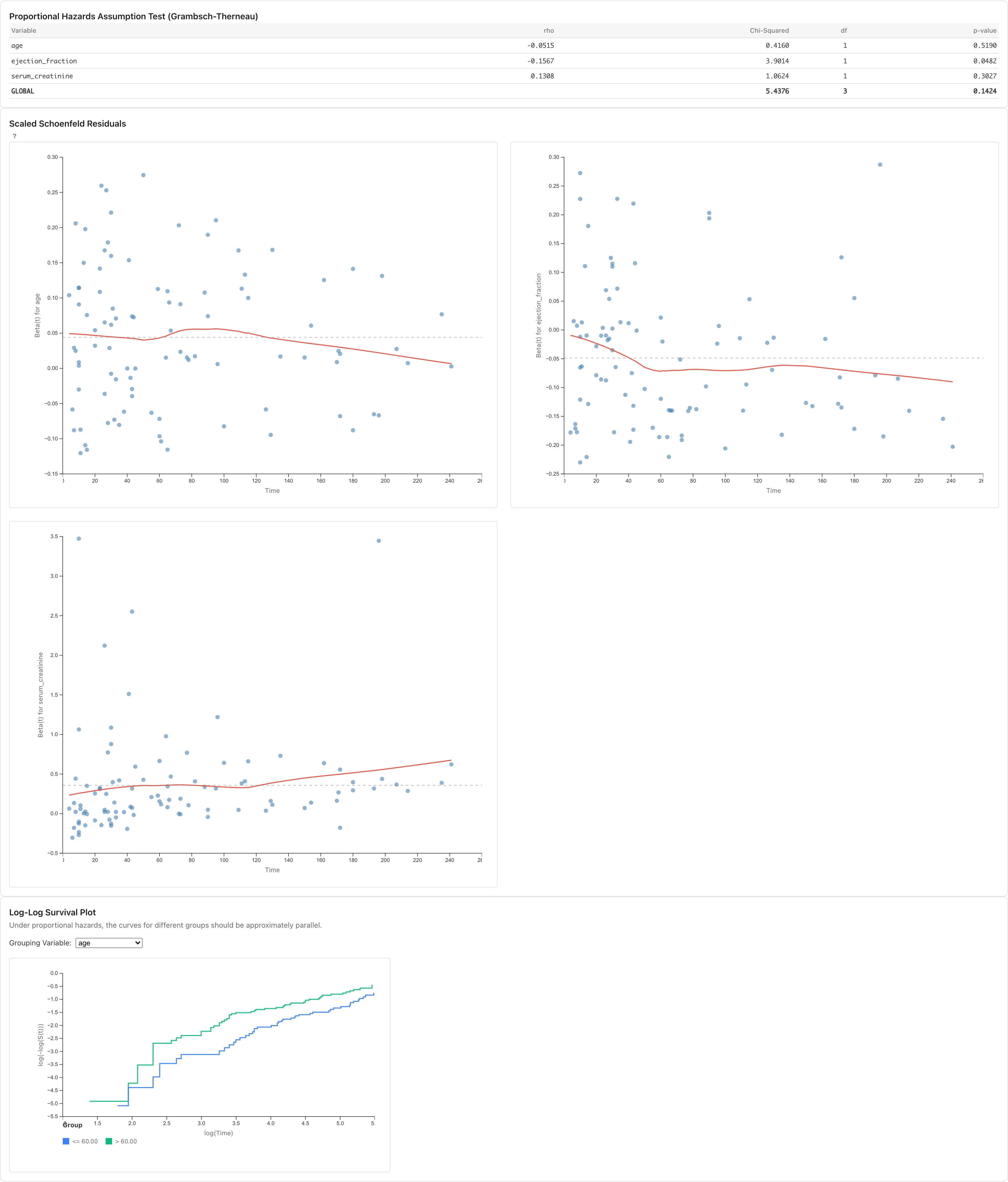
Below the coefficients table and model fit statistics, MIDAS displays diagnostics for the proportional hazards assumption. The Cox model assumes that covariate effects are constant over time — this is the proportional hazards assumption (details). When it breaks down, $\beta$ can only be interpreted as a weighted average over time.

Proportional Hazards Diagnostics

Displays the correlation between scaled Schoenfeld residuals and time for each covariate (Grambsch & Therneau, 1994). Uses the KM time transformation $g(t) = 1 - \hat{S}(t^-)$ .

Column	Description
Variable	Variable name
rho	Pearson correlation between scaled Schoenfeld residuals and a Kaplan-Meier-based time transform. Values close to 0 are consistent with the assumption

Covariates with a large absolute rho may have effects that change over time. Since rho alone does not reveal the pattern or severity of the departure, inspect the Schoenfeld residual plots below. MIDAS uses rho together with visual inspection of the plots, and does not display a test statistic or p-value.

Scaled Schoenfeld Residuals

For each covariate, plots scaled Schoenfeld residuals against time. The red curve is a LOESS smooth; the dashed gray line is the estimated coefficient $\hat\beta$ . Under proportional hazards, residuals scatter randomly around $\hat\beta$ and the LOESS line stays close to horizontal. An upward or downward trend in the LOESS line indicates that the covariate's effect varies over time.

Log-Log Survival Plot

Plots group-specific Kaplan-Meier estimates as $\log(-\log(\hat{S}(t)))$ versus $\log(t)$ . Select the grouping covariate from the Grouping Variable dropdown. When the selected covariate has five or fewer distinct values, each value forms its own group; with six or more, observations are split into two groups at the median. The median split is a convenience that discards some information from the continuous variable and may miss (or exaggerate) non-proportionality at the continuous scale. For continuous covariates, the Schoenfeld residual plot above is better suited for diagnosing the proportional hazards assumption. Under proportional hazards, the curves are approximately parallel. Curves that cross or change their separation over time suggest a violation.

When the diagnostics above suggest a violation of the proportional hazards assumption, approaches such as stratified Cox models or time-dependent covariate models can address it, but MIDAS does not currently support them. Interpret results with care, considering the severity of the violation and the goals of the analysis. If the goal is to compare groups defined by a single categorical variable, Kaplan-Meier with RMST is an alternative that does not rely on the proportional hazards assumption, although it cannot adjust for covariates.

Notes

Tied events (multiple events at the same time) are handled using the Efron method (details)
When convergence fails, the results show Convergence: No. Coefficient estimates may be unstable; consider reducing the number of covariates or rescaling covariates
Rows with missing values in the time, event, or any covariate variable are automatically excluded (listwise deletion; see Missing Data Mechanisms for validity conditions). When rows are excluded, the results show the number of excluded rows as "N rows excluded due to missing values."

References

Grambsch, P. M. and Therneau, T. M. (1994). Proportional hazards tests and diagnostics based on weighted residuals. Biometrika, 81(3), 515--526. https://www.jstor.org/stable/2337123

Also available as a Markdown file.

Survival Analysis

Data Requirements

Kaplan-Meier

Basic Usage

Understanding Results

Survival Curve

Summary Statistics

Number at Risk

RMST (Restricted Mean Survival Time)

Restriction Time τ\tauτ

Group Differences

Notes

Adding to Reports

Cox Regression

Basic Usage

Understanding Results

Cox Proportional Hazards Regression

Adjusted Survival Curve

Baseline Cumulative Hazard

Proportional Hazards Diagnostics

Proportional Hazards Diagnostics

Scaled Schoenfeld Residuals

Log-Log Survival Plot

Notes

See also

References

Restriction Time $\tau$