Generalized Linear Model (GLM)

The GLM tab performs regression analysis using generalized linear models. A GLM is defined by a distribution family, a linear predictor $\eta = X\beta + \text{offset}$, and a link function $g(\mu) = \eta$, extending OLS to the exponential family of distributions. The offset term defaults to zero when not specified. See GLM Fundamentals for the mathematical background.

OLS regression in the Linear Regression tab is a special case of GLM (Gaussian family with identity link). See Linear Regression for details on OLS.

Distribution Families and Link Functions

The distribution families and link functions available in MIDAS are listed below.

Choosing a Distribution Family

Family	UI Label	Variance Function $V(\mu)$	Use Case
Gaussian	Gaussian (Normal)	$1$	Continuous response variable. Equivalent to standard linear regression
Binomial	Binomial (Logistic)	$\mu(1 - \mu)$	Binary data (0/1) or proportion data. Logistic regression
Poisson	Poisson (Count)	$\mu$	Count data (event occurrences). Assumes variance equals the mean
Gamma	Gamma (Positive Continuous)	$\mu^2$	Positive continuous values with right-skewed distributions (wait times, costs)
Negative Binomial	Negative Binomial (Overdispersed Count)	$\mu + \mu^2/\theta$	Overdispersed count data. Use when the Poisson equidispersion assumption $\operatorname{Var}(Y) = \mu$ does not hold

The choice of family is driven by the nature of the response variable. Binary outcomes call for Binomial, non-negative integers for Poisson (or Negative Binomial if overdispersed), and positive continuous values with variance proportional to the mean for Gamma.

The Binomial family supports both individual 0/1 data (Binary) and aggregated successes/trials data (Grouped). See Grouped Binomial GLM with Dose-Response Data for details.

Link Functions

The link function is a monotonic function $\eta = g(\mu)$ connecting the linear predictor to the expected value of the response. Except for Negative Binomial, each family's default link is its canonical link. The canonical link for Negative Binomial is $\log(\mu/(\mu+\theta))$, but when $\theta$ is estimated the link function changes at each iteration, making estimation unstable. Log is used as the default in practice.

Family	Default Link	Available Links
Gaussian	Identity	Identity, Log
Binomial	Logit	Logit, Probit
Poisson	Log	Log, Identity
Gamma	Inverse	Inverse, Log, Identity
Negative Binomial	Log	Log

Link Function	Formula	Description
Identity	$\eta = \mu$	No transformation. Canonical link for Gaussian
Logit	$\eta = \log\!\bigl(\mu / (1 - \mu)\bigr)$	Log-odds transformation. Canonical link for Binomial
Log	$\eta = \log(\mu)$	Log transformation. Canonical link for Poisson. Ensures $\mu > 0$
Inverse	$\eta = 1/\mu$	Reciprocal transformation. Canonical link for Gamma
Probit	$\eta = \Phi^{-1}(\mu)$	Inverse CDF of the standard normal distribution. Corresponds to a latent normal variable model

The canonical link provides stable maximum likelihood estimation. Non-canonical links may be chosen for easier coefficient interpretation but can lead to convergence issues. See GLM Fundamentals for the mathematical properties of canonical links.

Basic Usage

The examples below use the Auto MPG dataset.

Opening GLM

Select Analysis > Generalized Linear Model (GLM)... from the menu bar.

Setting Up Variables

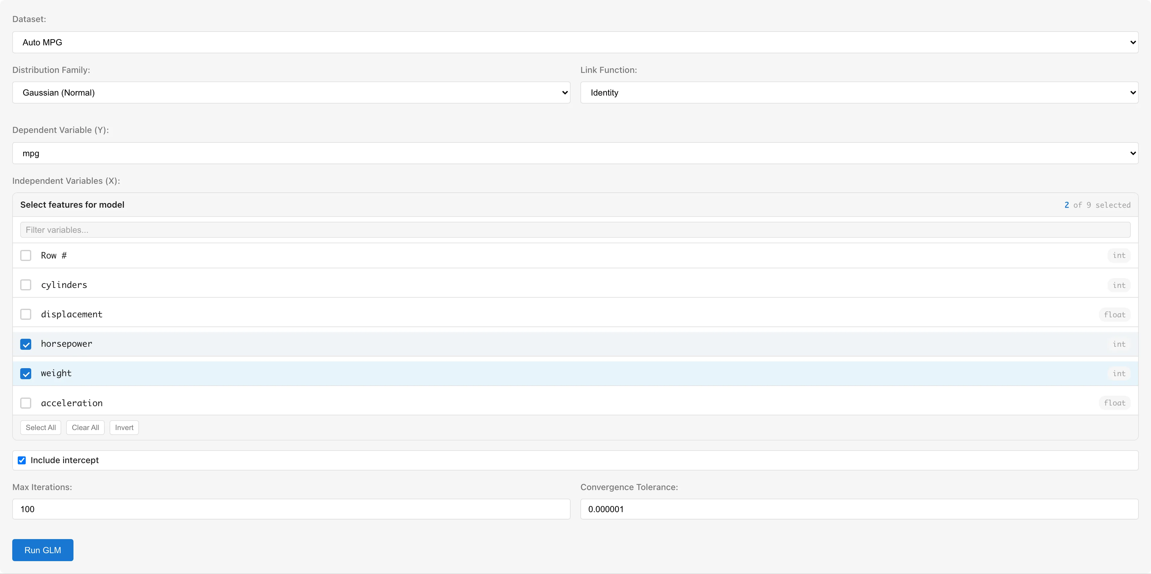
Dataset selects the dataset to analyze.

Dependent Variable (Y) selects the response variable. Numeric columns (int64, float64) and boolean columns are available. Boolean values are automatically converted to true=1, false=0. For the Binomial family, use a 0/1 or boolean column.

Independent Variables (X) selects predictor variables using checkboxes. Columns with categorical scales (nominal/ordinal) or date/datetime types are not selectable. To use categorical variables, convert them to numeric dummy variables using the Dummy Coding tab first (see Notes).

Distribution Family selects the distribution family. Changing the family automatically switches the link function to the canonical link for that family.

Link Function selects the link function. Available options depend on the selected family.

Include intercept toggles the intercept term. Enabled by default.

Negative Binomial Settings

When the Negative Binomial family is selected, options for the shape parameter $\theta$ appear. The Negative Binomial variance is $\operatorname{Var}(Y) = \mu + \mu^2/\theta$, where $\theta$ controls the degree of overdispersion.

• Automatic (default): $\theta$ is estimated using profile likelihood. An outer loop optimizes $\theta$ while an inner IRLS loop estimates $\beta$
• Manual: Check Manually specify θ and enter a value (0.1 to 100, default 1.0). Useful for sensitivity analysis or model comparison

Interpreting $\theta$:

• $\theta \to \infty$: Converges to Poisson ($\operatorname{Var}(Y) \to \mu$)
• $\theta \approx 10\text{--}100$: Moderate overdispersion
• $\theta \approx 1\text{--}10$: Strong overdispersion
• $\theta < 1$: Extreme overdispersion

Offset Variable

Offset Variable adds a known quantity to the linear predictor with a fixed coefficient of 1. The offset is not estimated from data; it is a fixed value for each observation.

A typical use case is rate modeling in Poisson regression. Set the count as the response variable and $\log(\text{exposure})$ as the offset to model rates instead of counts:

$\eta_i = X_i\beta + \log(\text{exposure}_i)$

This parameterization means that $\exp(\beta)$ is interpretable as a rate ratio.

Setting an offset also affects the null deviance. The null model becomes intercept + offset, so the null deviance differs from the case without an offset.

When predicting with a saved model that includes an offset, the prediction dataset must contain an offset column with the same name. The linear predictor for prediction is $\hat\eta_i = X_i\hat\beta + \text{offset}_i$.

Advanced Options

• Max Iterations: Maximum number of IRLS iterations (default: 100)
• Convergence Tolerance: Convergence threshold based on maximum absolute change in coefficients (default: 1e-6)

Running the Analysis

Click the Run GLM button.

Parameter estimation uses IRLS (Iteratively Reweighted Least Squares; see algorithm details). The progress dialog shows the deviance at each iteration. Click Cancel to stop the analysis, and use Save as Dataset to save the convergence history.

Understanding Results

Model Summary

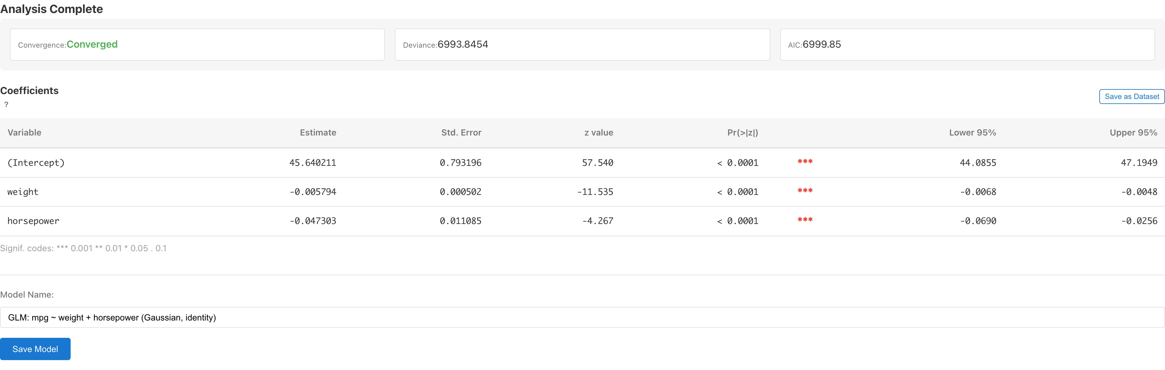
Metric	Description
Convergence	Whether IRLS converged (with iteration count)
Deviance	Residual deviance $D = 2\bigl[\ell(y;\,y) - \ell(y;\,\hat\mu)\bigr]$. A goodness-of-fit measure based on the log-likelihood difference from the saturated model
AIC	Akaike Information Criterion $\text{AIC} = -2\ell + 2k$, where $k$ is the total number of estimated parameters. Used for comparing models within the same family. Comparing AIC across different families is not recommended because the constant terms in the log-likelihood differ. Lower values indicate better fit-complexity trade-off
Shape Parameter ($\theta$)	Negative Binomial only. $\theta$ controls the degree of overdispersion: smaller values indicate stronger overdispersion, while $\theta \to \infty$ converges to Poisson (see Negative Binomial Settings). Indicates whether $\theta$ was estimated or manually specified

$k$ in the AIC formula is the number of regression coefficients (including the intercept). When $\theta$ is automatically estimated for Negative Binomial, $\theta$ is included in $k$ ($k = \text{number of regression coefficients} + 1$). When $\theta$ is manually specified, it is not included because it is not an estimated parameter. Be aware of this difference when comparing AIC between $\theta$-estimated and $\theta$-fixed models.

Coefficients

Column	Description
Variable	Variable name (intercept shown as "(Intercept)")
Estimate	Estimated regression coefficient $\hat\beta$ (on link function scale)
Std. Error	Wald standard error $\sqrt{\hat\phi \cdot \operatorname{diag}\bigl((X'\hat WX)^{-1}\bigr)}$. $\hat\phi$ is the dispersion parameter ($\hat\phi = 1$ for Poisson, Binomial, and Negative Binomial with estimated $\theta$)
z value / t value	Test statistic $\hat\beta / \operatorname{SE}(\hat\beta)$. For families that estimate the dispersion parameter $\phi$ from data (Gaussian, Gamma, Negative Binomial with fixed $\theta$), the reference distribution is $t(n-p)$ and the column header displays "t value". For families with $\phi = 1$ (Poisson, Binomial, Negative Binomial with estimated $\theta$), the reference distribution is standard normal and the column header displays "z value". Except for Gaussian + Identity, the test statistic follows the reference distribution only approximately in finite samples
Pr(>|z|) / Pr(>|t|)	Two-sided p-value. Based on the $t$-distribution for dispersion-estimating families, or the standard normal distribution for others
Lower N% / Upper N%	Confidence interval $\hat\beta \pm c \times \operatorname{SE}(\hat\beta)$, where N is the selected confidence level. $c$ is $t_{1-\alpha/2,\, n-p}$ for dispersion-estimating families, or $z_{1-\alpha/2}$ for others (e.g., $z_{0.975} = 1.96$ at the 95% level)

For Gaussian + Identity, the test statistic follows $t(n-p)$ exactly when errors are normally distributed. For other dispersion-estimating families (Gaussian with non-identity link, Gamma, Negative Binomial with fixed $\theta$), the $t$-distribution is an approximation that accounts for the additional uncertainty from estimating $\phi$. For families with known dispersion ($\phi = 1$), the Wald test is an asymptotic approximation to the standard normal. Neither approximation is exact in finite samples; both improve as the sample size grows. Interpret results near borderline significance levels (p-values around 0.05) with caution.

For Negative Binomial with estimated $\theta$, $\phi = 1$ because the overdispersion is already modeled by the $\mu^2/\theta$ term in the variance function — there is no remaining overdispersion for $\phi$ to absorb, so standard errors are computed with $\phi = 1$. When $\theta$ is manually fixed, the specified value may not fully capture the data's overdispersion, so $\hat\phi = \text{Pearson }\chi^2/(n-p)$ is estimated instead. This follows R's MASS::glm.nb.

Interpreting Coefficients

Coefficients are estimated on the link function scale, so interpretation requires considering the inverse link function.

• Identity link: $\beta$ is the change in $E[Y]$ per unit change in $X$ (same as OLS)
• Logit link: $\beta$ is the change in log-odds. $\exp(\beta)$ is the odds ratio
• Log link: $\beta$ is the change in $\log(\mu)$. $\exp(\beta)$ is the multiplicative change in $E[Y]$ (rate ratio)
• Inverse / Probit link: Direct interpretation is difficult; interpretation through predicted values is more practical

The coefficients table can be saved as a dataset using the Save as Dataset button for export to CSV. You must save the model first (using the Save Model button). Linking the coefficient dataset to a specific model means that deleting the model also deletes the derived coefficient dataset and any report element that references it, and refitting the model updates the dataset contents to reflect the new fit.

In the saved dataset, column names differ from the UI labels: z value / t value is saved as Test Statistic and Pr(>|z|) / Pr(>|t|) as P-value. The saved dataset also includes a Distribution column (value: normal or t) and a DF column. When Distribution is normal, DF is empty.

Saving and Diagnostics

Saving the Model

Enter a model name in the Model Name field and click Save Model. The model name defaults to the format "GLM: Y ~ X1 + X2 (Family, link)".

If an existing model with the same configuration (dataset, response variable, predictor variables, family, link function) exists, a confirmation dialog for overwriting is displayed.

Data Generated on Save

Saving a model automatically creates a derived dataset that adds diagnostic columns to the original data.

Column	Symbol	Description
fitted_values	$\hat\mu_i = g^{-1}(x_i'\hat\beta)$	Predicted values (on the response scale)
deviance_residuals	$d_i$	Deviance residuals
pearson_residuals	$r_i = (y_i - \hat\mu_i) / \sqrt{V(\hat\mu_i) / w_i}$	Pearson residuals. $w_i$ is the prior weight ($w_i = 1$ for binary data)
standardized_residuals	$r_i^* = d_i / \sqrt{\phi(1 - h_i)}$	Standardized residuals (deviance-based)
leverage	$h_i$	Leverage (diagonal of the hat matrix)
cooks_distance	$D_i$	Cook's Distance

The $\phi$ used for computing standardized residuals and Cook's Distance differs by family. For Poisson, Binomial, and Negative Binomial, $\phi = 1$: the variance function $V(\mu)$ specifies the theoretical variance, so overdispersion is not absorbed into the diagnostic statistics. For Negative Binomial, $\phi = 1$ regardless of whether $\theta$ is estimated or fixed. For Gaussian, $\phi = \text{Deviance}/(n - p)$; for Gamma, $\phi = \text{Pearson }\chi^2/(n-p)$. This follows R's stats::glm and MASS::glm.nb. Note that for Negative Binomial with fixed $\theta$, this differs from the $\hat\phi = \text{Pearson }\chi^2/(n-p)$ used for standard errors in the coefficients table.

Diagnostics and Details

After saving the model, two buttons appear:

• View Model Details - Opens the Model Detail tab showing detailed model information
• View Diagnostics - Opens the GLM Diagnostics tab showing diagnostic plots

Diagnostic Plots

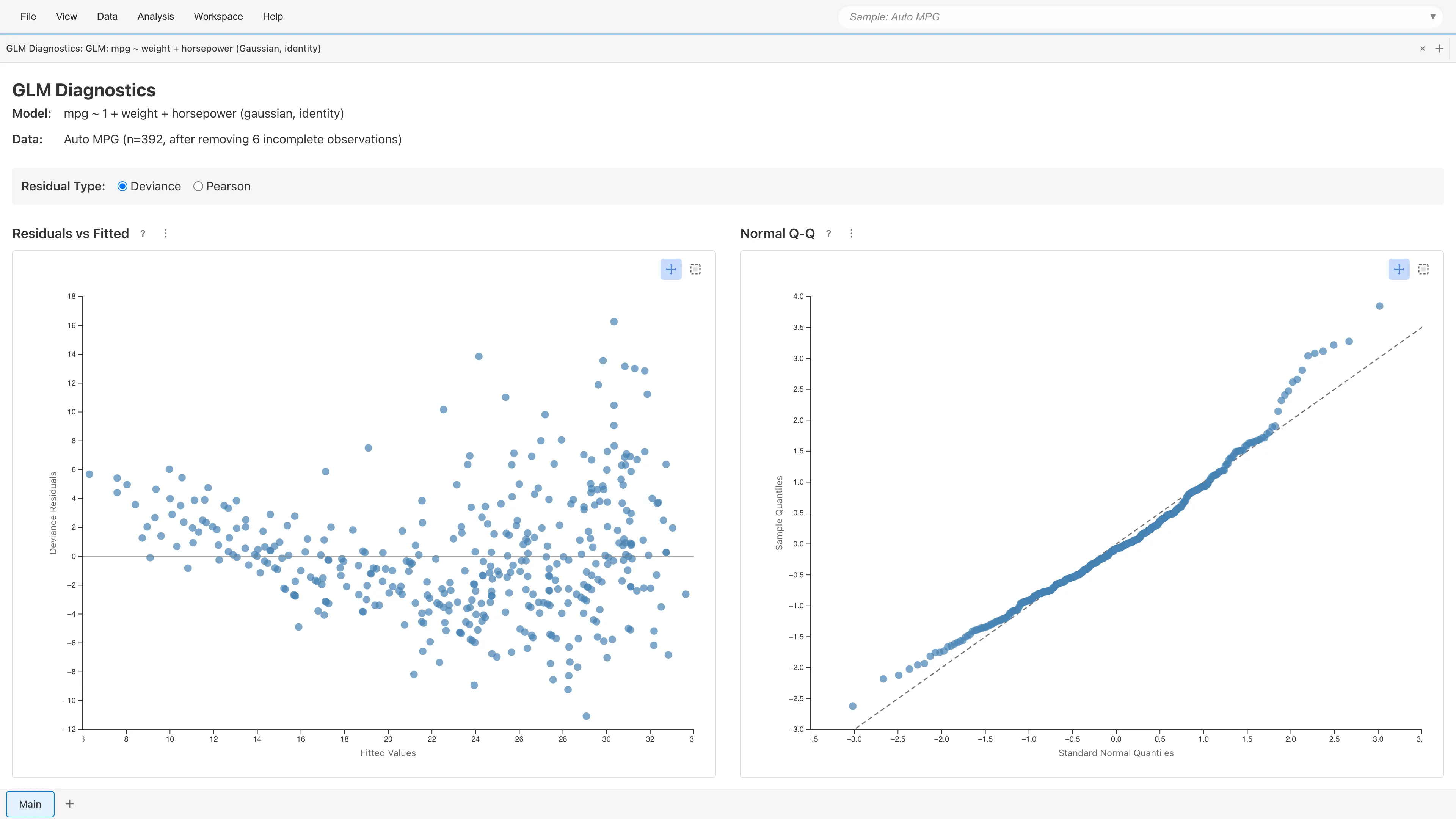
Clicking View Diagnostics displays four diagnostic plots. As with OLS, check linearity, constant variance, and outlier influence.

Residual Type Selection

Select the residual type: Deviance (default) or Pearson. Switching updates all four plots immediately.

• Deviance Residuals: $d_i = \operatorname{sign}(y_i - \hat\mu_i) \times \sqrt{2\bigl[\ell(y_i;\,y_i) - \ell(y_i;\,\hat\mu_i)\bigr]}$, where $\ell(y_i; y_i)$ is the log-likelihood under the saturated model ($\mu_i = y_i$). Likelihood-based residuals and the default in MIDAS
• Pearson Residuals: $r_i = (y_i - \hat\mu_i) / \sqrt{V(\hat\mu_i) / w_i}$. $w_i$ is the prior weight ($w_i = 1$ for binary data; $w_i$ is the number of trials for grouped Binomial). Observed-minus-expected scaled by the variance function. Useful for diagnosing overdispersion, as Pearson $\chi^2 = \sum r_i^2$ is used to estimate the dispersion parameter $\phi$

Residuals vs Fitted

Plots residuals against fitted values $\hat\mu$. Random scatter around zero indicates adequate model fit.

• Curved pattern: The link function may be inappropriate, or nonlinear effects of predictors may be missing
• Funnel-shaped pattern: The variance function may be inappropriate (e.g., Poisson's $\operatorname{Var} = \mu$ does not match the data)

Normal Q-Q Plot

Shown only for Gaussian family. Plots standardized residual quantiles against theoretical normal quantiles.

For non-Gaussian families, deviance residuals are not guaranteed to be asymptotically normal (particularly for binary Binomial data). Instead of the plot, the message "This plot is only shown for Gaussian family GLMs." is displayed.

Scale-Location

Plots $\sqrt{|\text{standardized residuals}|}$ against fitted values. Constant variance is indicated by points spreading evenly in the horizontal direction.

An upward trend suggests variance depends on fitted values. Since GLM explicitly models the mean-variance relationship through the variance function $V(\mu)$, patterns in this plot suggest the chosen family's variance function does not match the data well.

Residuals vs Leverage

Plots standardized residuals against leverage $h_i = \operatorname{diag}(H)_i$ (diagonal elements of the hat matrix). Cook's (1977) distance contours are displayed at $D = 0.5$ (orange dashed) and $D = 1.0$ (red dashed).

• Leverage: Measures how far an observation's predictor values are from others. $h_i > 2p/n$ ($p$ = number of parameters, $n$ = number of observations) indicates high leverage
• Cook's Distance: $D_i = \dfrac{r_i^{*2}}{p} \cdot \dfrac{h_i}{1 - h_i}$. $D_i > 0.5$ warrants attention; $D_i > 1.0$ indicates strong influence

Observations outside the contour lines may substantially change the model estimates if removed.

Point Selection

Click or rectangle-select data points on any plot to display details (fitted values, residuals, leverage, Cook's Distance, etc.) in a table below the plots. Selection state is synchronized across all four plots.

Deviance Goodness-of-Fit

For Poisson and Binomial families, the residual deviance approximately follows a $\chi^2(n - p)$ distribution when the model is correctly specified. The Deviance Goodness-of-Fit chart displays the $\chi^2$ density curve and marks the observed deviance, allowing you to visually assess whether the deviance falls within the bulk of the distribution or in the extreme tail.

A deviance in the right tail suggests the model does not adequately capture the variability in the data. Consider whether important predictors are missing or whether the distributional assumption is appropriate. For Poisson data, switching to the Negative Binomial family may help. See GLM Fundamentals for the theoretical background.

For Binomial models with binary response data (trial size = 1), the assumptions for the $\chi^2$ approximation are not met, so this test is unreliable. Use the other diagnostic plots to assess model fit in that case.

Prediction

Use a saved GLM model to generate predictions on new data.

Running Predictions

1. Open the Model Detail tab via View Model Details
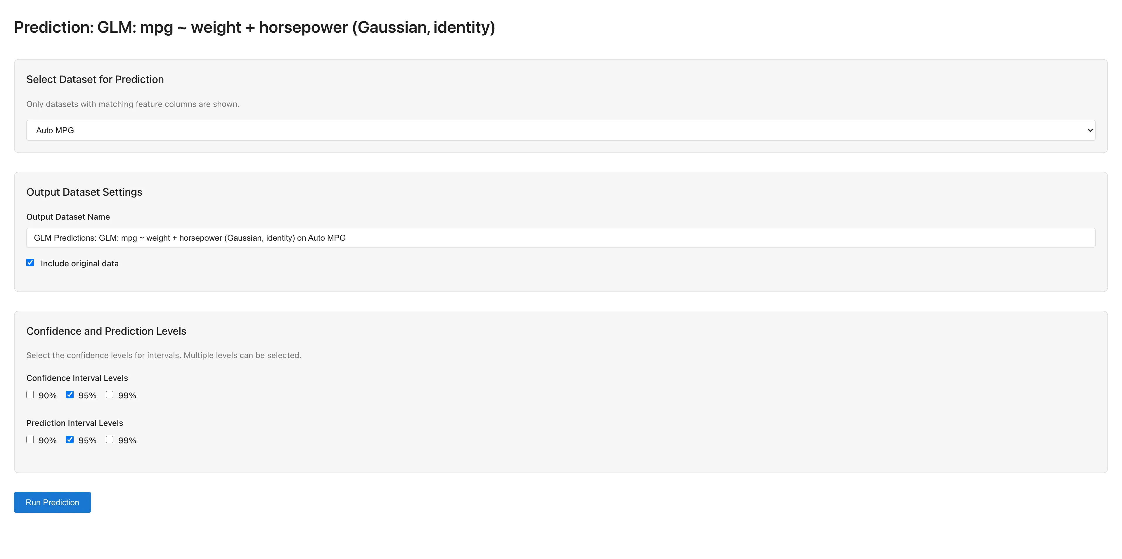
2. Click the Make Predictions button to open the GLM Prediction tab
3. Select a dataset for prediction (only datasets with matching predictor column names are available)
4. Configure output settings:
   • Output Dataset Name: Name for the prediction results dataset
   • Include original data: Whether to include original columns in the output
   • Confidence Interval Levels: Confidence interval levels (90%, 95%, 99%)
   • Prediction Interval Levels: Prediction interval levels (90%, 95%, 99%)
5. Click Run Prediction to execute

Prediction Output

Prediction results are saved as a dataset containing:

• Predicted values $\hat\mu = g^{-1}(X\hat\beta)$ (on the response scale)
• Confidence intervals for the mean response $E[Y \mid X]$, which capture the uncertainty in estimating the population mean at a given set of predictor values
• Prediction intervals for a new observation $Y_\text{new}$, which capture the uncertainty in a single future value including observation-level variability

Reference Distribution for Intervals

For families that estimate the dispersion parameter $\phi$ from data (Gaussian with any link, Gamma, Negative Binomial with fixed $\theta$), confidence and prediction intervals use the $t$ distribution with $n - p$ degrees of freedom, where $n$ is the number of training observations and $p$ is the total number of estimated parameters including the intercept. For Gaussian with identity link, this is the exact finite-sample result under the assumption that the errors are normally distributed. For other dispersion-estimating families, the $t$-distribution accounts for the additional uncertainty from estimating $\phi$.

For families with known dispersion ($\phi = 1$: Poisson, Binomial, Negative Binomial with estimated $\theta$), intervals use the standard normal ($z$) distribution as the reference. This is an asymptotic approximation that becomes more accurate as the sample size increases.

The reference distribution and degrees of freedom are displayed in the Prediction tab.

Prediction Interval Methods

Prediction interval computation depends on the family. Gaussian with identity link uses an analytical formula that includes estimation uncertainty, while other combinations use plug-in methods. Plug-in methods do not account for parameter estimation uncertainty, so coverage probability may fall below the stated confidence level in small samples or for extrapolation points. See GLM Fundamentals for the formulas.

When the prediction dataset contains the response variable, accuracy metrics (R², RMSE, MAE) are automatically calculated and displayed.

Notes

Using Categorical Variables

GLM only accepts numeric variables. To use categorical (nominal/ordinal) or date/datetime variables as predictors, convert them to numeric dummy variables using the Dummy Coding tab before running the analysis.

Automatic Exclusion of Missing and Invalid Values

Rows containing missing values (null), non-numeric values, or infinity are automatically excluded from the analysis. The number of excluded rows is displayed in the Model Summary.

Convergence Issues

If IRLS fails to converge, check the following:

• Iteration count: Increase Max Iterations (e.g., 100 → 500)
• Tolerance: Relax Convergence Tolerance (e.g., 1e-6 → 1e-4)
• Scaling: Large differences in predictor scales can cause numerical instability. Consider standardizing
• Perfect separation: In logistic regression, when a predictor perfectly separates the response classes, the maximum likelihood estimate does not converge to a finite value (Albert & Anderson, 1984). Remove the offending predictor or verify the data
• Excess zeros: When count data contains an extreme number of zeros, Poisson or Negative Binomial models may struggle to fit adequately

References

• Nelder, J. A., & Wedderburn, R. W. M. (1972). Generalized linear models. Journal of the Royal Statistical Society: Series A, 135(3), 370-384. https://www.jstor.org/stable/2344614
• Cook, R. D. (1977). Detection of influential observation in linear regression. Technometrics, 19(1), 15-18. https://www.jstor.org/stable/1268249
• Albert, A., & Anderson, J. A. (1984). On the existence of maximum likelihood estimates in logistic regression models. Biometrika, 71(1), 1-10. https://www.jstor.org/stable/2336390