The DoE Analysis Tab

The DoE Analysis tab analyzes 2-level factorial experiment data. It supports orthogonal array generation, estimation of factor effects through main effects plots and interaction plots, and decomposition of variation through ANOVA tables.

Open the Tab

Select Analysis > DoE Analysis... from the menu bar.

Generate an Orthogonal Array

Click New Design... in the top-right corner of the DoE Analysis tab.

Define Factors

Enter a name and two level labels for each factor. At least 2 factors are required.

Array Type

Select an orthogonal array type based on the number of factors.

Orthogonal arrays are generated from Hadamard matrices. Every pair of factors has balanced level combinations, and factors are uncorrelated in the design matrix.

When the number of factors is at most log2(runs), the generated plan is a full factorial containing every level combination. This covers 2 factors on L4, up to 3 factors on L8, and up to 4 factors on L16. When the number of factors is below log2(runs), each level combination appears runs / 2^factors times even with Replications = 1.

When the number of factors exceeds log2(runs), some effects become confounded. With 5 factors on L16, neither main effects nor two-factor interactions are confounded with each other. With 4 factors on L8 and 6 to 8 factors on L16, main effects are confounded neither with each other nor with two-factor interactions, but two-factor interactions are confounded with each other. With 3 factors on L4, 5 or more on L8, and 9 or more on L16, main effects are confounded with two-factor interactions, so main effects are estimated under the assumption that interactions are negligible.

Max Factors is the upper limit on how many factors can be placed in the array, not necessarily the number of factors that can be analyzed without replication. See the next section on replication.

Replications

Set the number of replications in the Replications field. The default is 1. When set to 2 or more, each row in the orthogonal array is duplicated the specified number of times. For example, L4 with Replications = 3 generates 4 base rows x 3 replications = 12 rows.

Adding replications increases the number of observations and improves the precision of the error variance estimate. When the number of observations is less than or equal to the number of parameters, the error variance cannot be estimated and running the analysis produces an error. For example, an L4 with 3 factors and main effects only has 4 parameters including the intercept against only 4 observations. Add replicates or choose an array type with more runs than needed.

Randomization

Randomize run order is on by default and shuffles the experimental conditions. Randomization prevents systematic bias from run order, so leaving it on is recommended for actual experiments. Turn it off to keep the orthogonal array's row order.

Generate the Dataset

After previewing the array, click Generate to add it as a dataset. The response column is created empty. To enter your experimental results, select Edit Data from the table menu in the top-right corner of the data table.

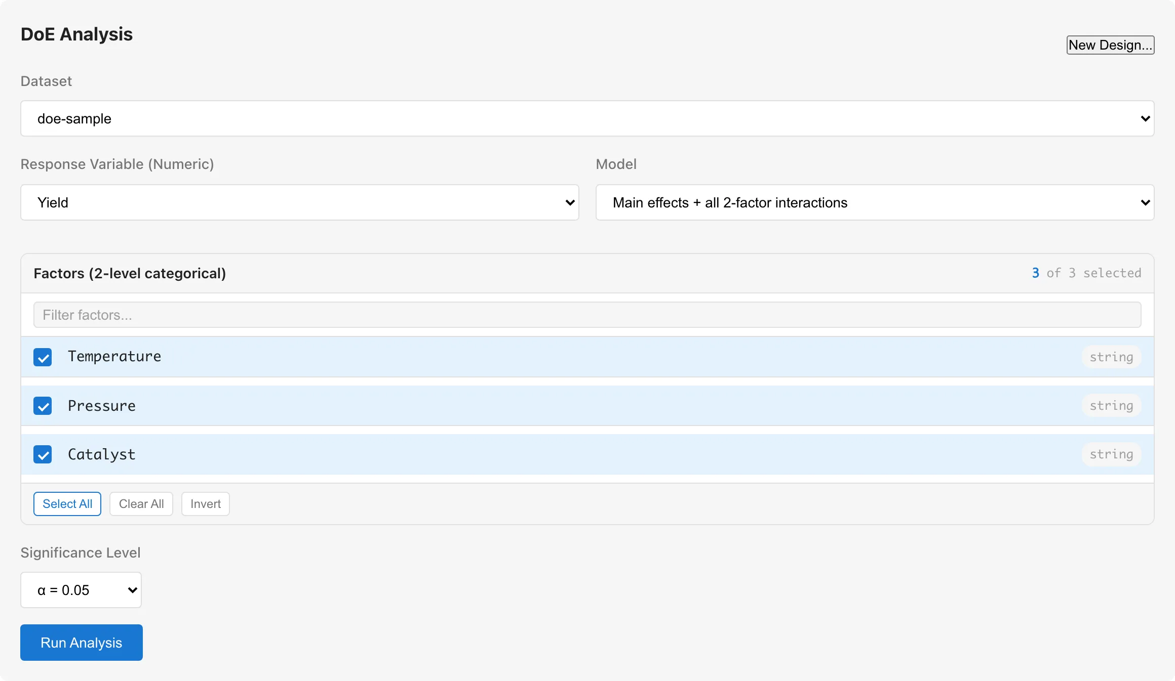
Run an Analysis

Configure the following in the settings panel, from top to bottom. Response Variable and Model sit side by side on the same row.

1. Select a dataset from Dataset
2. Select a numeric variable for Response Variable (Numeric)
3. Choose a Model type
4. Select 2-level categorical variables under Factors (categorical) (at least 2)
5. Click Run Analysis

Data Requirements

Factors must be categorical variables. Columns with nominal or ordinal measurement scale appear as factor candidates. The current version supports only 2-level factors. Selecting a factor with 3 or more levels produces an error message when you run the analysis.

Select a numeric column for the response variable.

Model Selection

Main effects only: Includes only the main effect of each factor. Use this when interactions between factors can be assumed negligible.

Main effects + all 2-factor interactions: Adds all pairwise 2-factor interaction terms to the main effects. Use this when interactions may be present. More factors mean more interaction terms and fewer residual degrees of freedom. For example, selecting all 7 factors from an L8 with all 2-factor interactions requires 7 main effects + 21 interactions + intercept = 29 parameters, but only 8 rows of data are available. Start with main effects only and add interactions as needed.

Main effects + selected interactions: Adds only the interaction terms you select.

Reading the Results

Results are displayed across five sub-tabs (ANOVA Table / Effects / Main Effects / Interaction / Diagnostics).

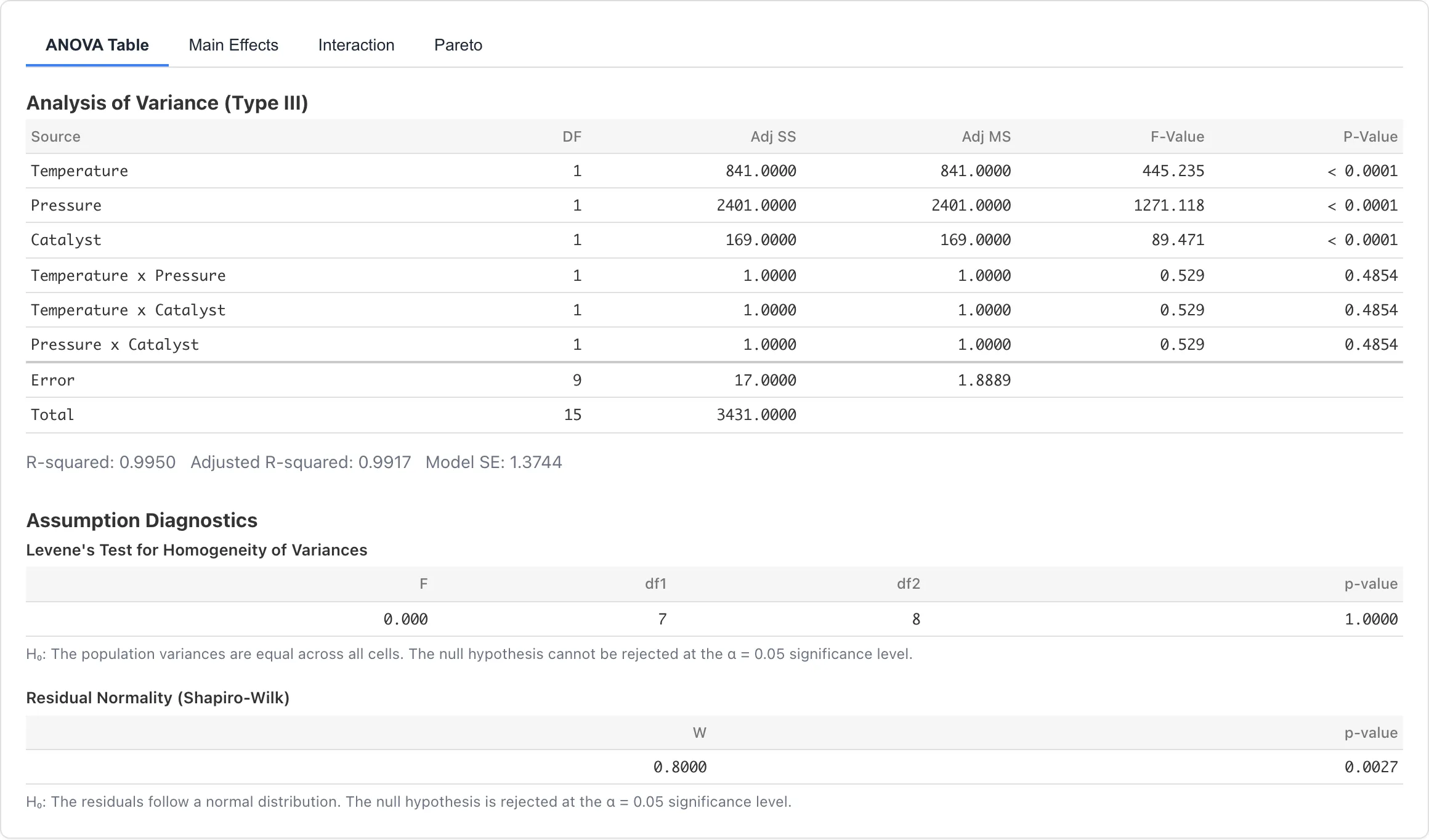
ANOVA Table

Shows sums of squares and effect size estimates for each factor and interaction, using Type III sums of squares.

R-squared, Adjusted R-squared, and Model SE are shown below the table.

When the variation in the response is below floating-point precision relative to its magnitude, the sum-of-squares decomposition is meaningless. This covers responses whose values are all identical, as well as responses with a tiny relative spread on top of a large offset. R-squared, the partial η²/ω² estimates, and each term's sum of squares are then undefined and shown as "-", and a warning explains why. The Std. Error column of the Factor Effects table and the error bars on the main effects plot are likewise undefined.

Click a row to highlight the corresponding factor in the main effects or interaction plots.

Factor Effects

Shows the point estimate, standard error, and confidence interval of the effect for each term (main effects and interactions, excluding the intercept). Test statistics and p-values are not shown.

Effects are least-squares estimates. They match the difference of observed level means for balanced designs but not for unbalanced designs. The (level A − level B) shown in a main effect's Term means the effect is the mean at level A minus the mean at level B. Which level is the +1 reference is determined by the effect coding rule.

The confidence interval depends on the fitted model and its assumptions; its width reflects the precision of the effect estimate.

Use the Add to Report button to add the factor effects table to a report.

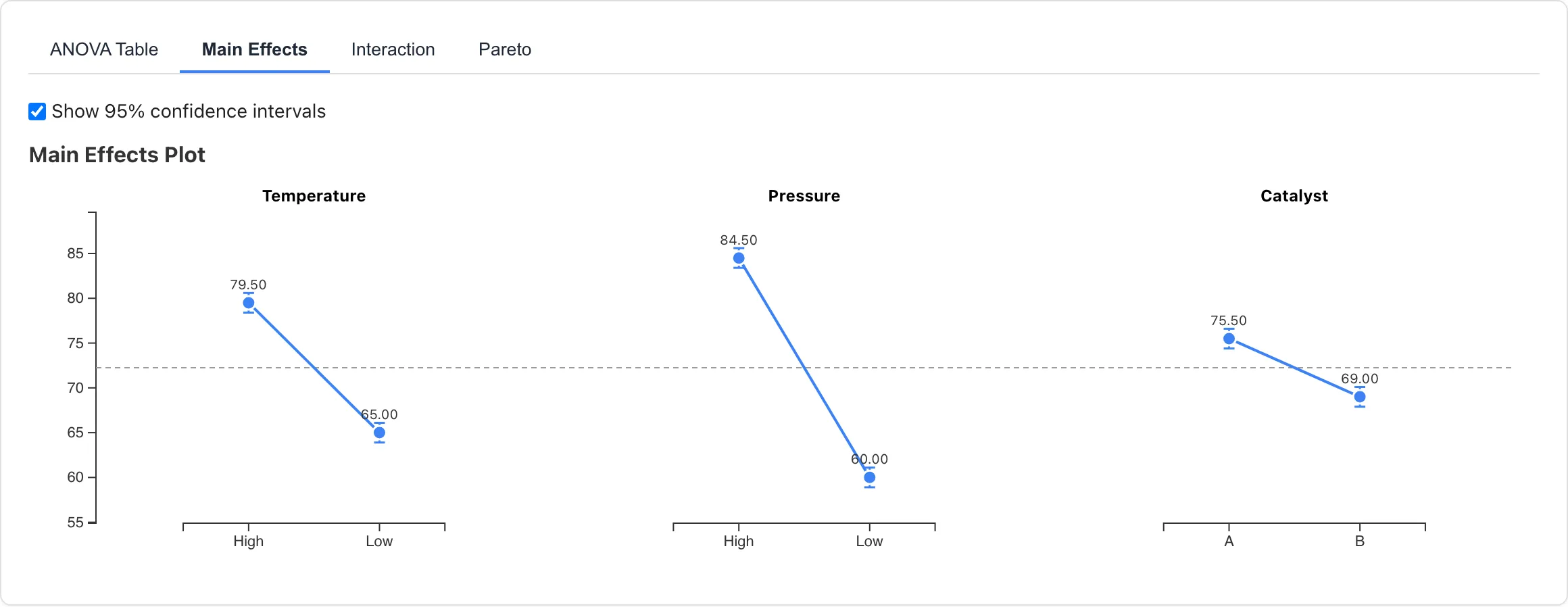
Main Effects Plot

Displays the observed mean response at each level of each factor as a line chart. Each factor gets its own subplot, and the Y-axis scale is shared across all subplots. A steeper slope indicates a larger effect on the response.

The horizontal dashed line represents the grand mean. The grand mean is the intercept of the OLS model, which equals the arithmetic mean of all observations in a balanced design.

Enable Show 95% confidence intervals to display error bars for each level mean. The confidence level is fixed at 95%. The standard error is $\text{SE} = \sqrt{\text{MSE} / n_i}$ where MSE is the residual mean square from the fitted model and $n_i$ is the number of observations at that level. This standard error uses the pooled residual variance from the entire model, which assumes equal error variance across all levels. Interval width uses the t-distribution critical value based on the residual degrees of freedom. These error bars show the precision of individual level mean estimates and serve a different purpose from testing differences between levels. For a degenerate response, whose variation is below floating-point precision, MSE is undefined and the error bars are not shown.

Click a point to select the corresponding rows in the data table.

Click Add to Report to add the main effects plot to a report.

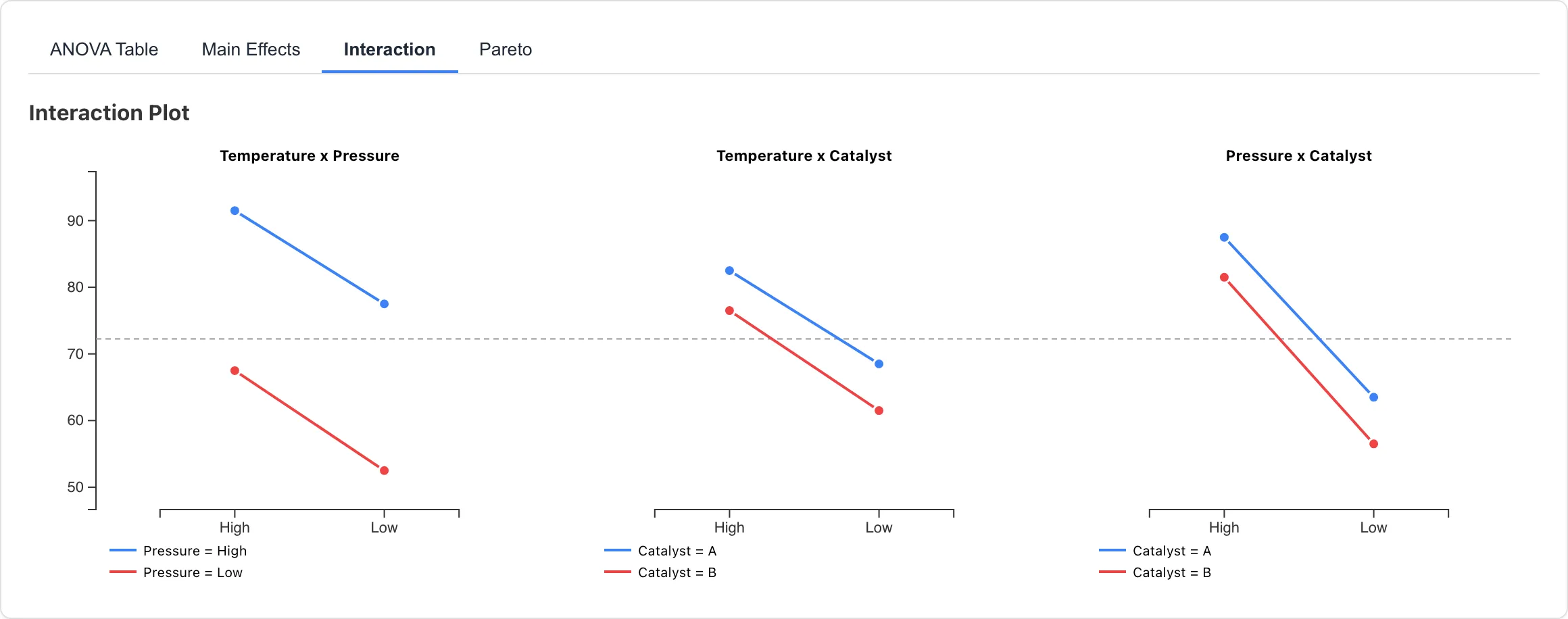
Interaction Plot

Shows cell means as a line subplot for each interaction pair included in the model. The X-axis represents one factor, and color-coded lines represent the levels of the other factor. With Main effects + all 2-factor interactions, $\binom{n}{2}$ subplots are drawn for $n$ factors. With Main effects + selected interactions, only the selected pairs are drawn. With Main effects only, this tab shows no subplots.

Lines that are nearly parallel suggest little interaction. Crossing lines indicate that one factor's effect depends on the level of the other factor. The ANOVA Table's effect size columns (partial η², partial ω²) provide a quantitative assessment of interaction magnitude.

Click a point to select the corresponding cell's rows in the data table.

Click Add to Report to add the interaction plot to a report.

Diagnostics

Displays a residual Q-Q plot. The residuals are computed as $y_i - \hat{y}_i$, where $\hat{y}_i$ is the fitted value from the OLS model.

Systematic departures from the reference line indicate non-normality of residuals: heavy tails appear as upward/downward curvature at the ends, skew appears as an S-curve, and outliers appear as isolated points far from the line.

This tab checks the normality assumption only. Homogeneity of variance should be assessed separately by comparing the spread of responses across factor level combinations.

Click Add to Report to add the residual Q-Q plot to a report.

Statistical Model

Effect Coding

Each 2-level factor is coded as +1 for the first level (alphabetically) and -1 for the second level. Because the two levels are placed at ±1, the regression coefficient equals half the difference in mean response between levels. The main effects plot shows the mean response at each level with its confidence interval. Level labels appear in alphabetical order on the X-axis, so the left level corresponds to +1 and the right level to -1. SS and effect sizes do not depend on the coding direction, but the sign of the regression coefficient is positive when the +1 level has a higher mean response.

Interaction columns are the element-wise product of the corresponding main effect columns.

Estimation

A design matrix including the intercept and all terms is constructed, and coefficients are estimated by ordinary least squares via Householder QR decomposition.

Type III Sums of Squares

Each factor's sum of squares is computed as $\text{SS}_j = t_j^2 \times \text{MSE}$, where $t_j = \hat\beta_j / \text{SE}(\hat\beta_j)$ is the ratio of each coefficient in the full model to its standard error. Since each 2-level factor has 1 degree of freedom, this value equals the Type III sum of squares. This evaluates each factor's unique contribution after adjusting for all other factors, independent of the order in which factors are entered. See ANOVA for more on Type III sums of squares. DoE Analysis uses effect coding, while the ANOVA page describes interpretation based on treatment coding. The coefficient meanings differ, but for balanced 2-level orthogonal arrays the sums of squares and effect size decomposition are identical regardless of the coding.

Assumptions

This analysis assumes:

• Independence: Each experimental run is conducted independently
• Normality: The error in the response variable follows a normal distribution
• Homogeneity of variance: The error variance is equal across all factor level combinations

Independence is determined by how the experiment was conducted. Normality can be assessed using the residual Q-Q plot in the Diagnostics tab. Homogeneity of variance can be assessed by comparing the spread of responses across factor level combinations.

Missing Values

Rows with missing values (null), empty or blank cells, non-numeric values, or infinity in any factor or the response variable are excluded from the analysis. The number of excluded rows is shown in the results panel. This exclusion is listwise deletion; see Missing Data Mechanisms for conditions under which it yields valid estimates.

If your data was generated from an orthogonal array and rows are excluded, the design loses its orthogonality and the factors become correlated. Correlation between factors increases the standard errors of effect estimates. In addition, Type I and Type III sums of squares coincide for orthogonal data but diverge once the factors are correlated, meaning the individual sums of squares no longer add up to the model sum of squares.

The loss of orthogonality is reported in the results panel as an "Unbalanced design detected" warning. In that case, the cell means shown in the main effects and interaction plots are unadjusted observed averages, not least-squares means (estimated averages that adjust for the imbalance between factors). Their standard errors likewise receive no adjustment for the imbalance. The grand mean dashed line is the intercept of the OLS model, not the arithmetic mean of all observations.

If all observations for some factor combination are lost, an "Empty cells detected" warning also appears. The effect estimates then rely on the assumption that interactions excluded from the model are negligible, and the data cannot check this assumption for the empty combinations. Both "Unbalanced design detected" and "Empty cells detected" are warnings: the analysis still runs. Plan your experiments to minimize missing data.

If orthogonality breaks down enough that the design matrix becomes ill-conditioned, MIDAS shows a warning that the estimated condition number is high. This signals reduced numerical precision in the effect estimates. See Condition Number for what it means and how to address it.

Related Pages

• ANOVA -- One-way and two-way ANOVA without the 2-level restriction
• Linear Regression -- Regression analysis with continuous predictors

Also available as a Markdown file.