The Statistics Tab
The Statistics tab displays an overview of every column in the active dataset. The tab consists of two sections. The Columns section is a summary table with one row per column; clicking a row expands the details of that column right below it. The Relationships section is a grid of column pairs; clicking a cell shows the detail for that pair. Each section can be collapsed by clicking its heading.
The header displays the dataset name together with the row count (rows), the column count (cols), the number of selected columns (sel.), and the number of selected rows (rows sel.). When a filter is active, the row count takes the form "filtered rows / total rows", and statistics are computed on the filtered rows.
See also the "View Basic Statistics" section in Getting Started.
The Columns Section
The summary table displays every column, one row per column.
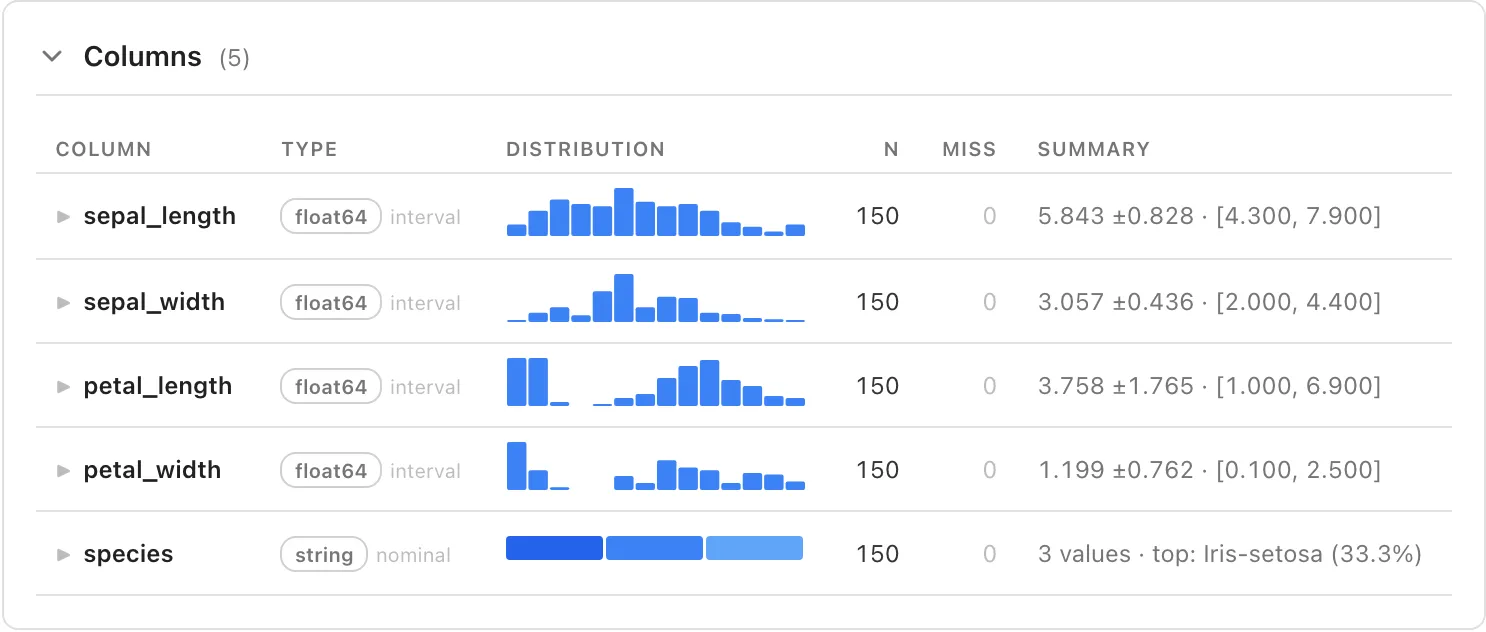
| Table column | Content |
|---|---|
| Column | Column name |
| Type | Data type and measurement scale |
| Distribution | Sparkline of the distribution |
| n | Non-null count |
| miss | Missing count |
| Summary | One-line summary suited to the type |
The sparkline in the Distribution column is a chart sized to fit the row, with no axes or ticks. Numeric and datetime columns show a histogram of bin counts; the other columns show a bar of the shares of the most frequent categories.
The content of the Summary column depends on the data type. Numeric columns with interval or ratio scale show "mean ±std [min, max]", numeric columns with nominal or ordinal scale show the most frequent value, string and Enum columns show the number of unique values and the share of the most frequent value, boolean columns show the counts and percentages of true / false, and datetime columns show the earliest and latest datetimes.
For datasets with many rows and columns, the statistics are computed one column at a time. The n, miss, and Summary cells of a column that has not been computed yet show "…" and are replaced with values as each column finishes. Computing every column in one go would leave the screen unresponsive, so the work is split up and the table stays readable while it fills in.
Expanding Column Details
Clicking a summary row expands the details of that column (distribution chart and statistics) right below the row. Clicking the row again collapses it.
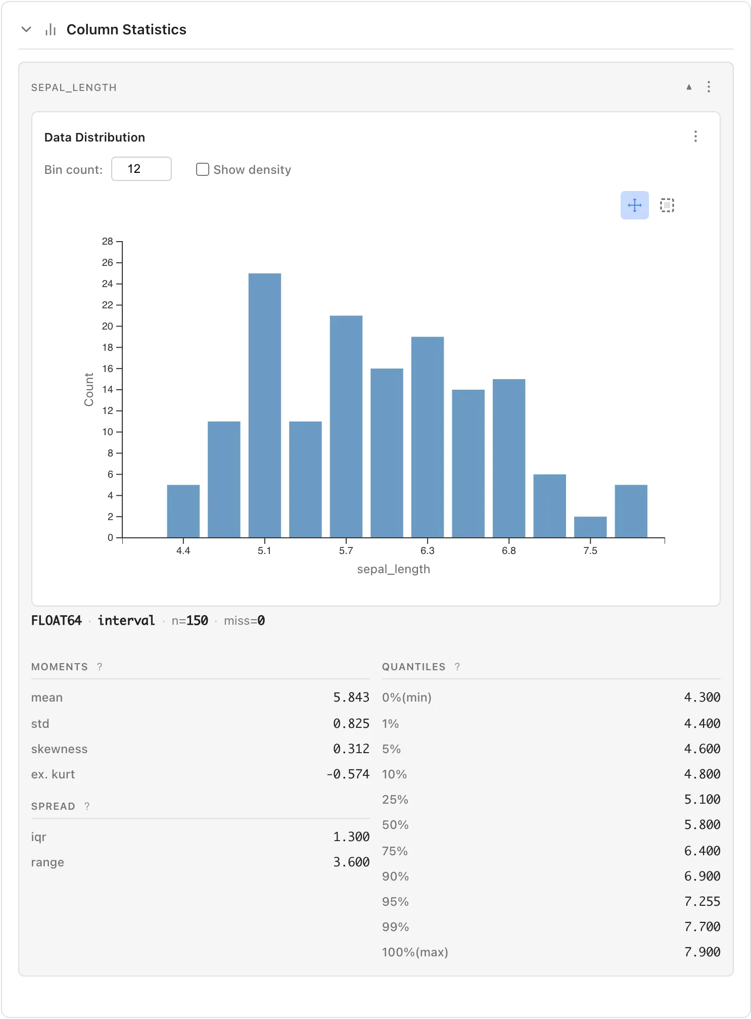
Expanding a row is the same operation as selecting the column. Expanded columns are highlighted in sync with the column selection in the Data Table, and columns selected via the Data Table column headers are also expanded in the Statistics tab. To view the expanded details at the full width of the pane, use the Selected Columns tab.
Statistics by Data Type
The content of the expanded details varies depending on the column's data type.
Numeric Type (int64, float64)
Measurement Scales and Displayed Statistics
For numeric types, MIDAS displays only statistically meaningful items based on the column's measurement scale (Nominal, Ordinal, Interval, Ratio).
| Statistic | Nominal | Ordinal | Interval | Ratio |
|---|---|---|---|---|
| Category breakdown (Most frequent) | o | o | ||
| min / max | o | o | o | |
| Quantiles (median, etc.) | o | o | o | |
| mean / std | o | o | ||
| skewness / ex. kurt | o | o | ||
| iqr / range | o | o |
For example, postal codes should be treated as Nominal scale. When treated as nominal, mean and standard deviation are not displayed because numerical magnitude has no meaning for nominal scales.
See Data Preparation and Import for how to change measurement scales.
For numeric columns with Nominal or Ordinal scale, a breakdown of counts per value (Most frequent) is displayed.
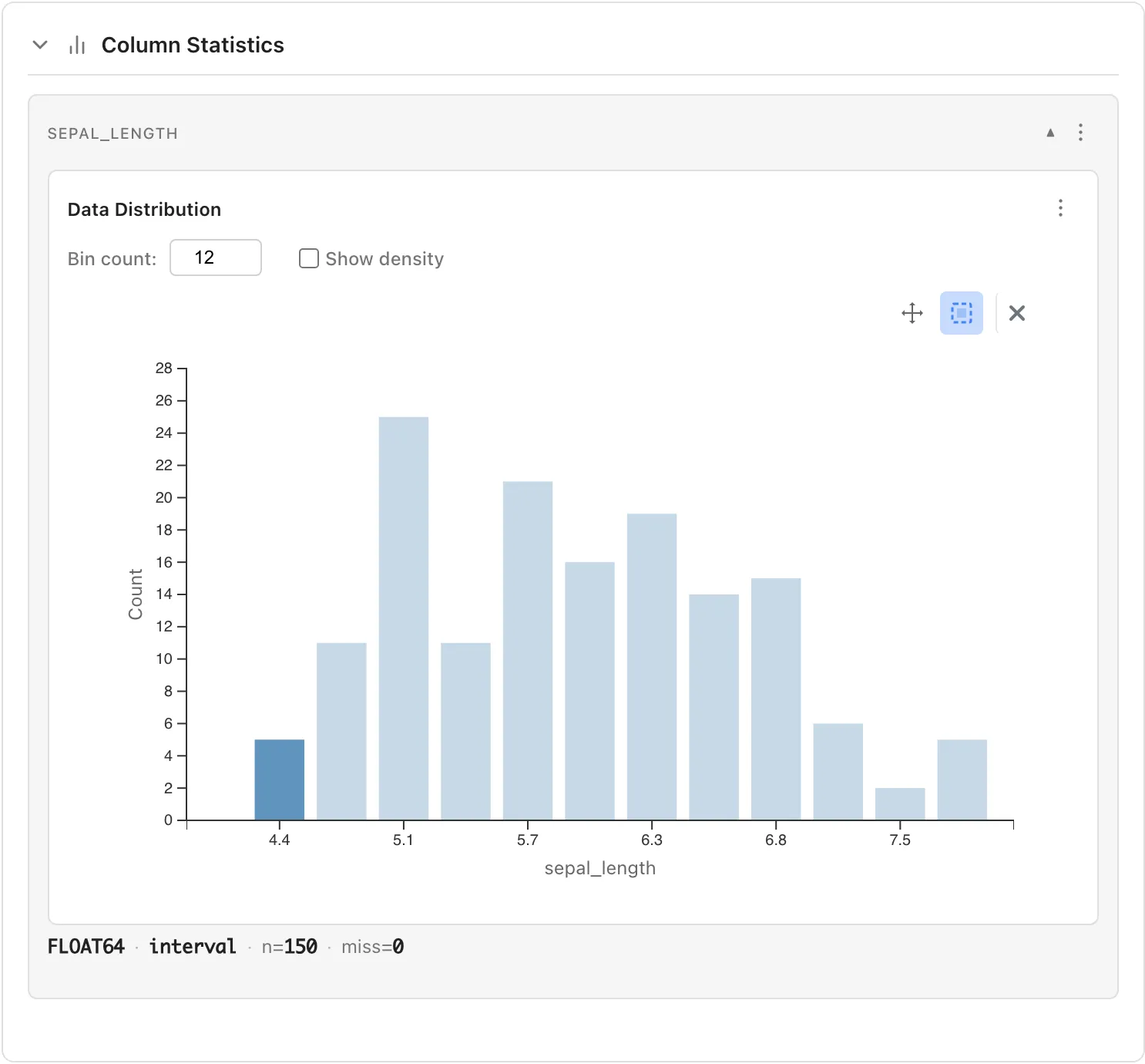
Data Distribution (Histogram)
Visualize the distribution of your data. For numeric columns with Nominal or Ordinal scale, a Category Distribution bar chart showing the count for each value is displayed instead of a histogram.
- Bin count: Adjust the number of histogram bins
- Y: Choose what the bar heights represent, Count or Proportion. Count is the number of rows and Proportion is the relative frequency, where the bar heights add up to 1
- Show density: When checked, overlays a kernel density estimation curve on the histogram
Use the buttons at the top right of the chart to switch operation modes:
- Pan mode: Drag to pan the chart
- Select mode: Drag to select a range and highlight corresponding rows
Moments
- mean: Average value
- std: Sample standard deviation ()
- skewness: Skewness where is the sample standard deviation defined above (bias-corrected, ). 0 indicates symmetry; positive values indicate a longer right tail, negative values a longer left tail
- ex. kurt: Excess kurtosis where is the sample standard deviation (bias-corrected, ). 0 indicates the same kurtosis as the normal distribution; positive values indicate heavier tails (values far from the mean occur more readily), negative values lighter tails
For columns with ratio scale, the following statistics are also displayed:
- cv: Coefficient of variation . Represents the relative magnitude of variability to the mean. Displayed only when the mean is positive (hidden for )
- geo mean: Geometric mean . Defined only when all values are strictly positive. Hidden for columns that contain zero or negative values
A column whose values span a range too wide to compute a statistic in double precision shows "N/A" in place of that statistic. This applies to the moments, the spread statistics, and interpolated quantiles. Rescale the column to get a value. A statistic that is not defined for the data at all is hidden instead of showing "N/A". std requires , skewness , and ex. kurt , and a constant column (zero variance) shows neither skewness nor ex. kurt.
Spread
- iqr: Interquartile range (75th percentile - 25th percentile)
- range: Range (maximum - minimum)
Quantiles
For numeric columns with interval or ratio scale, quantiles are calculated on the sorted data by computing and linearly interpolating as (R type 7). For ordinal columns (both numeric and Enum), quantiles are the -th value of the sorted data without interpolation (R type 1; for ), so the result is always an existing observed value. Shows positions when data is sorted in ascending order:
- 0%(min): Minimum value
- 1%, 5%, 10%: Lower percentiles
- 25%: First quartile
- 50%: Median
- 75%: Third quartile
- 90%, 95%, 99%: Upper percentiles
- 100%(max): Maximum value
String Type and Enum Type
Expanding a string or Enum column displays the following:
- Category Distribution: Bar chart showing count for each category
- Unique values: Number of unique values
- Most frequent: Most frequent values and their counts (click to select corresponding rows)
When an Enum column's measurement scale is changed to ordinal, min / max / median / Q1 / Q3 are also computed based on the position order of the Enum definition, in addition to the frequency counts above. mean / std / skewness / ex. kurt are not computed because ordinal categories do not have a defined distance. IQR (= Q3 − Q1) is also not computed because subtraction between category values is not defined. See The Manage Enums Tab for details.
Boolean Type
Expanding a True/False column displays the following:
- True: Count and percentage of True values
- False: Count and percentage of False values
Datetime Type
Expanding a datetime column displays the following:
- Date Distribution: Chart showing data distribution over time
- Interval: Select aggregation interval (Auto, 1 minute, 1 hour, 1 day, 1 week, 1 month, etc.)
- Show trend: Display trend line
- Earliest: The oldest datetime
- Latest: The most recent datetime
- Time span: Duration (e.g., "29 days, 22 hours")
The Relationships Section
The Relationships section displays a grid of column pairs. Cells for pairs of numeric columns show the Pearson correlation coefficient as both a number and a background color. The colors run from red (negative correlation) to blue (positive correlation), with a legend below the grid. Cells for pairs involving a categorical column, and cells for datetime × numeric pairs, show a glyph. Pairs of two datetime columns, or a datetime and a categorical column, are not supported and show "-".
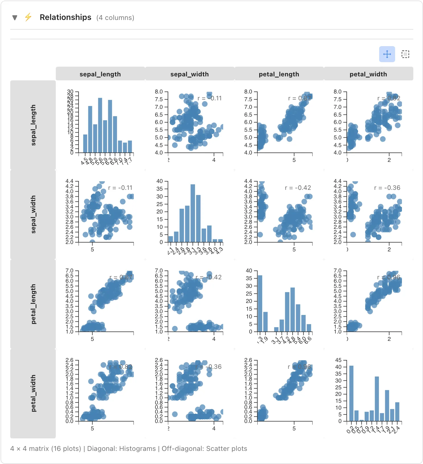
For datasets with more than 20 columns, the grid is limited to the first 20 columns and says so below the grid. This is because the number of correlations and cells grows with the square of the column count. To examine pairs beyond the first 20 columns, select just the columns of interest in the Selected Columns tab.
For datasets with many rows and columns, the correlations are computed alongside the rendering. Cells still being computed show "…", and "Computing correlations…" appears below the grid. The number of pairs grows with the square of the column count, so the rest of the screen stays usable while the computation runs. If the computation fails, "Correlations could not be computed." appears below the grid and the numeric cells show "-". Clicking a cell still opens the pair detail, which shows the correlation coefficient.
The correlation coefficient is computed using only the rows where neither column is missing, known as pairwise deletion. The number of rows used is shown as n in the cell tooltip and in the pair detail. When the missing values fall in different rows across columns, n differs from pair to pair.
The correlation obtained by pairwise deletion describes only the rows where both columns are observed. When missingness is related to the values themselves, as when values above a measurement limit are recorded as missing, the result can deviate systematically from the correlation that would be obtained if all rows were observed.
The Pearson correlation coefficient measures the strength of the linear relationship between two variables on a scale; note that it cannot capture nonlinear relationships (e.g., U-shaped relationships). It is also sensitive to outliers.
Pair Detail
Clicking a grid cell shows the detail for that pair right below the grid. Clicking the same cell again closes it. The content depends on the combination of columns. In this section, columns with Interval or Ratio scale are treated as numeric, and columns with Nominal or Ordinal scale are treated as categorical.
Numeric × Numeric -- Shows a scatter plot and the Pearson correlation coefficient. The number of rows used in the computation is shown next to the coefficient as n.
Categorical × Numeric -- Shows a chart of the numeric column by category. The Chart dropdown above the chart switches between a box plot for comparing distributions across categories (the default) and a bar chart of aggregated values. The box plot shows the median, quartiles, and whiskers; whiskers extend to the most extreme values within 1.5 × IQR of the quartiles, and values beyond the whiskers are drawn as individual points. For the bar chart, a dropdown sets the aggregation method (Sum, Average, Median, Min, or Max; Average is the default). The orientation (Horizontal or Vertical; Horizontal is the default) applies to both charts.
Categorical × Categorical -- Shows a cross tabulation (a table of row counts).
Datetime × Numeric -- Shows a line chart with the datetime column on the horizontal axis. Each row is drawn as a point on the line, and clicking a point selects that row.
Grouping Feature
Select a column from the Show stats by dropdown to switch the whole tab to a per-group view based on that column's values.
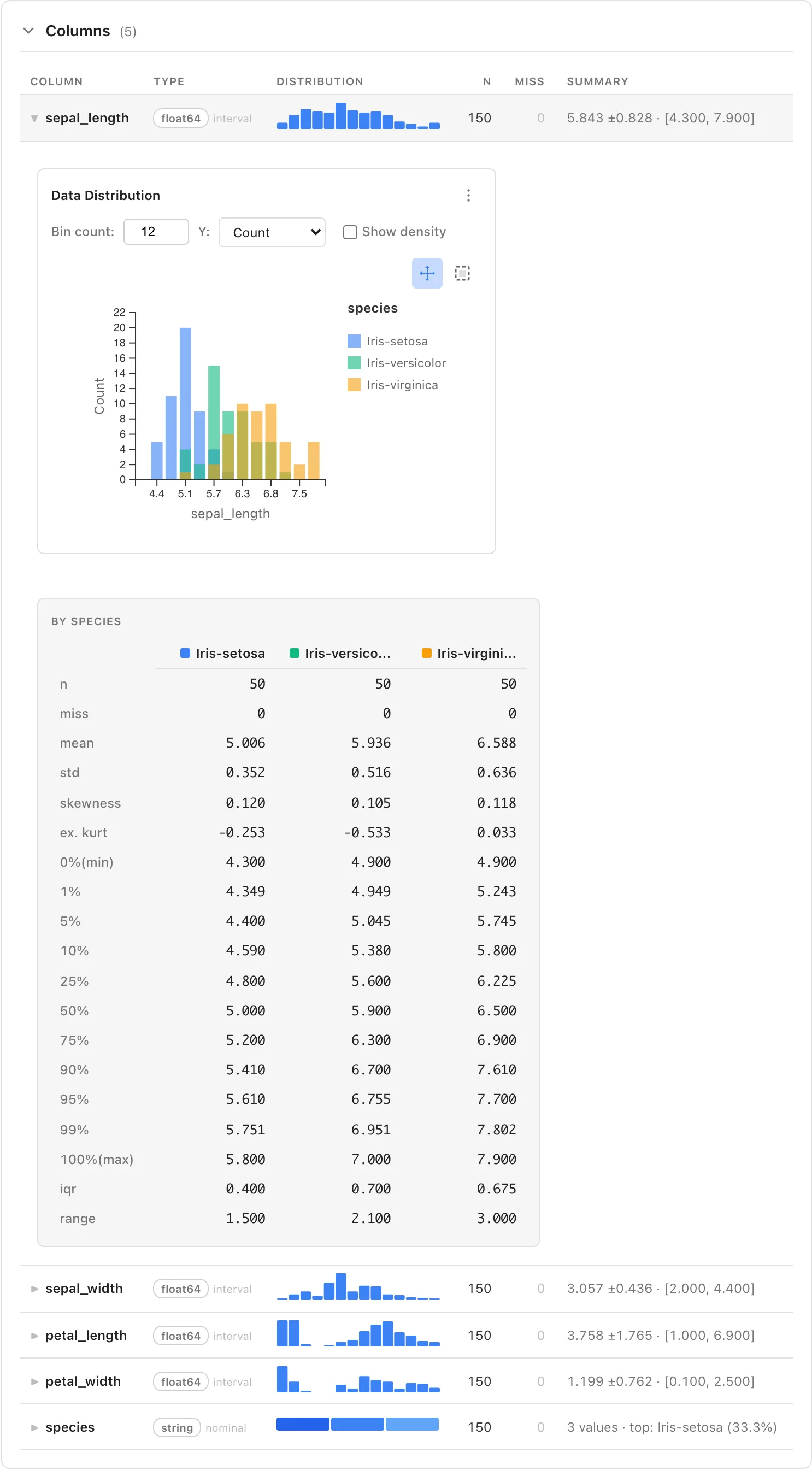
- Sparklines remain overall aggregates while grouping, regardless of column type. Expand a row to see the per-group breakdown
- The histogram in the expanded details of a numeric column becomes a per-group overlay. By default the bar heights are raw per-group counts, so when the groups differ in size, the height differences include the difference in row counts. Setting Y to Proportion makes each bar the relative frequency within its own group, which compares the shapes without the influence of the row counts. In a group with few rows, one row moves the proportion by a lot, so the bars swing correspondingly; read them together with the n row of the comparison table
- The Category Distribution in the expanded details of a column treated as categorical (string, Enum, and numeric columns with Nominal / Ordinal scale) remains an overall aggregate. The full breakdown is available in the cross tabulation of that column against the grouping column, shown in the same expanded details
- The Date Distribution histogram in the expanded details of a datetime column also remains an overall aggregate. The per-group earliest, latest, and span appear in the comparison table in the expanded details
- Statistics in the expanded details become a comparison table with one column per group
- Scatter plots in the pair detail are colored by group. The correlation coefficient shown next to them is computed on all rows ignoring the groups and is labeled "Pearson r (all rows, ignoring groups)"
- Rows whose value in the grouping column is missing are not included in any group. Their count is shown below the comparison table
- When the grouping column is an Enum, the order and colors of the groups follow the order of the Enum definition
Columns eligible for grouping are those of any type other than float64 with at most 20 unique values. Columns exceeding 20 appear in the dropdown but cannot be selected, because the overlays and the comparison table become unreadable beyond roughly that many groups.
Usage Example
In the Iris dataset, expanding the sepal_length column and grouping by species draws the distributions of Iris-setosa, Iris-versicolor, and Iris-virginica overlaid in a single histogram, and lines up statistics such as mean and std in a table with one column per species. You can compare the overlap of the distributions and the differences in the statistics on a single screen.
Row Selection Integration
You can select data rows from charts in the Statistics tab. See How Row Selection Works for an overview of how selection works across tabs.
Selection from Histogram
Click a bar: Click a histogram bar to select rows within that bin (range).
Rectangle selection: Switch to Select mode and drag to specify a range and select data within that area.
Adding to selection: Hold Ctrl (Mac: Cmd) while clicking to add to existing selection.
Selected rows are highlighted in the Data Table, and their count appears as rows sel. in the header.
Selection from Scatter Plot
In the pair detail scatter plot, click points to select rows. As with histograms, switching to Select mode with the buttons at the top right of the chart lets you drag to select points within a rectangular range.
Selection from Time Series Plot
In the time series plot shown in the datetime × numeric pair detail, click a point to select that row.
Selection from Categorical × Numeric Charts
In the bar chart and box plot displayed in the categorical × numeric pair detail, clicking a bar or a box selects all rows in that category. The box summarizes the whole category, so the selection also includes the rows drawn as points beyond the whiskers. Each point beyond the whiskers represents individual values, so clicking a point selects only the rows with that value.
Selection from Cross Tabulation
In the cross tabulations shown in the categorical × categorical pair detail and in the expanded details of categorical columns while grouping, clicking a cell selects the corresponding rows.
Opening Filtered Data Tab
Double-click a data point or bar in a chart, or a count in the Most frequent breakdown, to automatically open a Filtered Data tab displaying the corresponding rows.
Adding to Reports
The ⋮ button at the top right of the expanded details adds the column's statistics and histogram to a report. The categorical × numeric chart and the datetime × numeric time series plot in the pair detail can be added by right-clicking the chart. While grouping, only the histogram can be added, as it becomes a report element that keeps the per-group overlay.
See also
- The Selected Columns Tab -- Tab showing only the selected columns at full width
- How Row Selection Works -- How to select rows in each tab and how selection is shared
- Filtered Data -- Viewing rows behind double-clicked elements
- Data Types and Measurement Scales -- Statistical meaning of measurement scales
Also available as a Markdown file.