The Synthetic Data Generator Tab
The Synthetic Data Generator tab builds a dataset from a data generating process (DGP) in which every column declares a distribution. It lets you prepare regression, grouped, time-series, panel, and survival data without an external file. Because the true parameters used for generation are known, the data is useful for checking how an analysis method behaves and for practicing operations.
The same generation can also run through the Agent API's datasets.generateSynthetic. See Agent API for the JSON format of the spec, the options, and the error codes.
Generating Data
Choosing Data > Generate Synthetic Data... in the menu bar opens the tab.
In the form, enter Dataset name, Rows, and Seed, then list columns under Columns and choose a distribution and its parameters for each. Add Column adds a column, and the trash button at the end of a row removes it. Seed is an integer from −2,147,483,648 to 2,147,483,647. Rows is a positive integer up to 10,000,000.
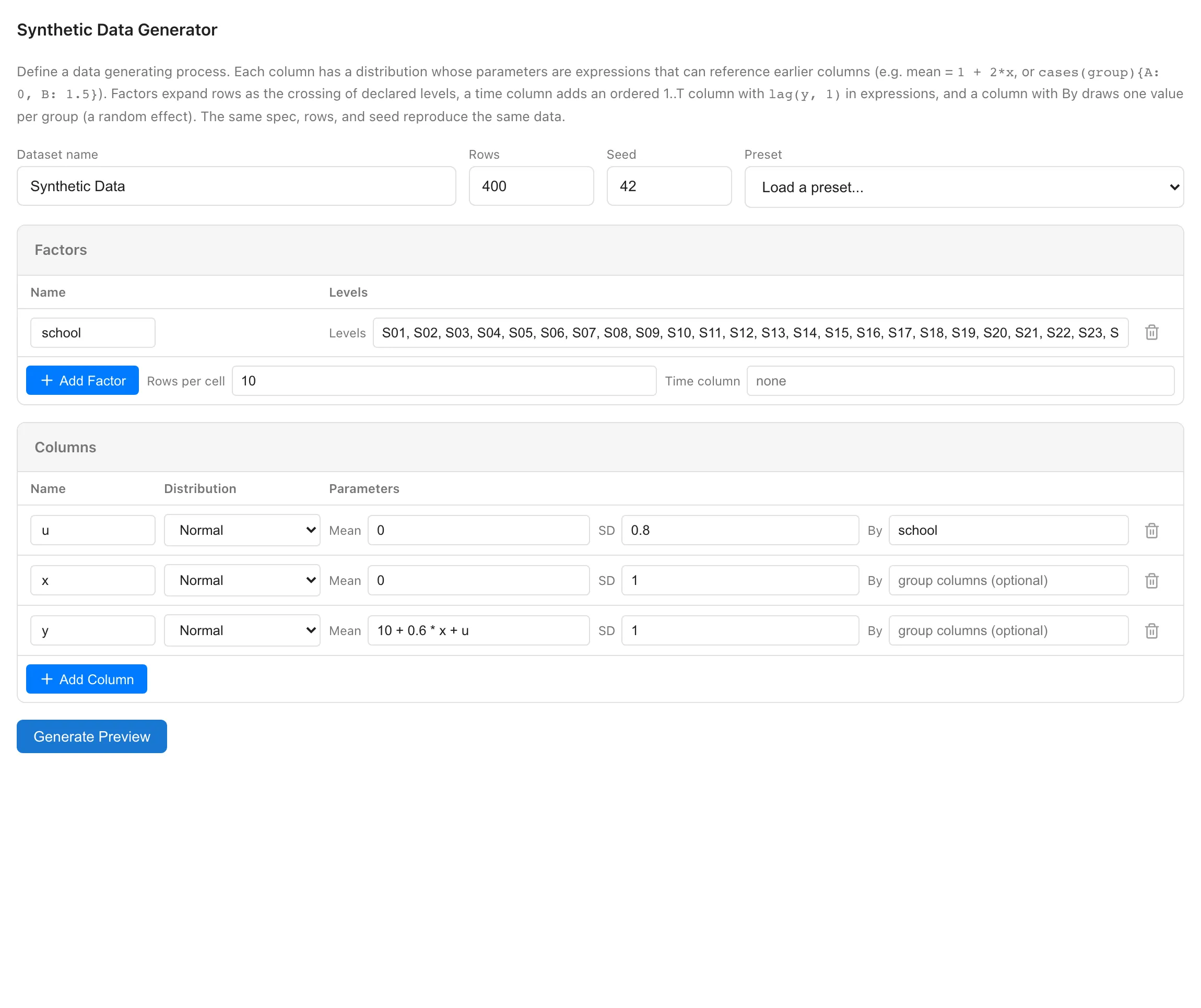
Generate Preview validates the input, generates the data, and shows the first 10 rows. When the input has an error, Generate Preview shows an error message and discards the previous preview.
Reviewing the Preview and Saving
Until you press Save as Dataset, no dataset is added to the project. Rerunning Generate Preview any number of times leaves existing datasets unchanged.
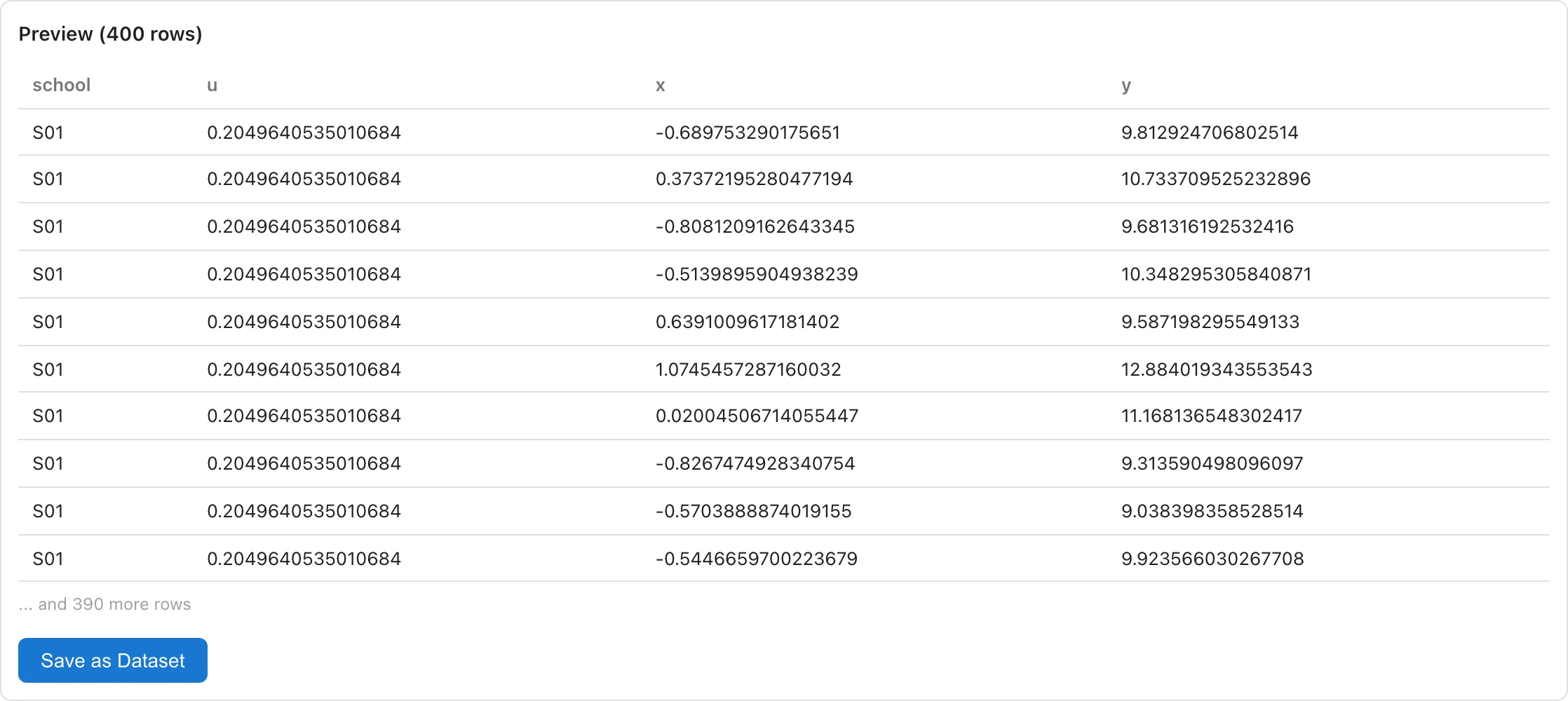
Pressing Save as Dataset creates the dataset, opens a Data Table tab, and closes the Synthetic Data Generator tab.
Saving under the same name as an existing dataset opens a dialog offering to rename, to append a number, or to replace. Replacing is available only when the target dataset was also created with the Synthetic Data Generator tab. Otherwise the dialog disables the replace option and explains why.
Columns and Distributions
Each column has one distribution. The distribution parameters are given as expressions. Expressions can reference other columns, so dependencies between columns express the generating process. See Expression Syntax for how to write them.
There are 8 distributions to choose from, and the parameter fields change with the distribution. The meaning of each parameter and the shape of each distribution are explained in Probability Distribution Fundamentals.
| Distribution | Parameters | Column data type |
|---|---|---|
| Normal | Mean, SD | float64 |
| Uniform | Min, Max | float64 |
| Bernoulli (0/1) | P | int64 |
| Categorical | Levels, Weights | string |
| Poisson | Lambda | int64 |
| Gamma | Shape, Scale | float64 |
| Weibull | Shape, Scale | float64 |
| Deterministic | Value | float641 |
Deterministic has no noise and writes the expression value directly into the column. Use it for a linear predictor column or a transformed copy of another column.
For Categorical, list the levels in Levels separated by commas and give a weight per level in Weights. Omitting Weights selects every level with equal probability. Each weight is itself an expression, so a weight can vary by row. MIDAS rejects negative weights and weights that are all zero. It also rejects a weight that evaluates to a non-finite value and weights whose sum is not finite.
Gamma and Weibull are parameterized by Shape and Scale. The mean of Gamma is Shape × Scale and its variance is Shape × Scale². The mean of Weibull is Scale × Γ(1 + 1/Shape), where Γ is the gamma function.
See Data Types and Measurement Scales for how column data types map to measurement scales.
When an expression evaluates to a value outside a parameter's domain, generation fails. Examples include an SD of Normal that is 0 or below, a Lambda of Poisson that is 0 or below, and a Max of Uniform that does not exceed Min2.
Every defined column becomes a column of the output dataset. There is no setting that excludes intermediate-calculation columns from the output.
Expression Syntax
An expression is text written in a distribution parameter, and it evaluates to a number.
An expression can reference other columns in the same definition by name. As long as the references have no cycle, the order of the columns does not matter. Numeric columns are referenced by writing their name directly. String columns (Categorical columns and the factor columns created by Add Factor) can only be referenced through cases, described below.
The available operators are the arithmetic operators + - * /, unary minus, and the comparisons < <= > >=. Precedence decreases from multiplication and division, to addition and subtraction, to comparisons, and parentheses make the order explicit. A comparison returns 1 when true and 0 when false3. Because the result is a number, a comparison can be multiplied with other terms and used as a 0/1 indicator variable.
Two comparisons cannot be written in a row as in mathematical notation, and 0 < x < 1 is a parse error. Intervals are written as a product of two comparisons, as in (0 < x) * (x < 1). = and == are not available4. Equality with a single value is also written as a product of two comparisons, as in (t >= 6) * (t <= 6).
The available functions and their argument counts are as follows.
| Function | Arguments | Meaning |
|---|---|---|
| exp(x) | 1 | exponential |
| log(x) | 1 | natural logarithm |
| sqrt(x) | 1 | square root |
| logistic(x) | 1 | logistic function 1/(1+exp(−x)) |
| pow(x, y) | 2 | power x^y |
| min(x, y) | 2 | smaller of two values |
| max(x, y) | 2 | larger of two values |
| abs(x) | 1 | absolute value |
cases switches the expression by the value of a string column. Write the referenced column name and an expression per level, as in cases(group){A: 0, B: 1.5, default: 0}. Either list every level or include a default entry. A level name can be written as is when it starts with a letter or _ followed by letters, digits, and _. Other level names are quoted, as in cases(group){"Group A": 0, default: 1}.
The return value of cases is the per-level value itself. Added to a base expression, as in 10 + cases(group){control: 0, treat: 1.5}, it expresses a per-group shift.
cases also maps levels to quantitative values. Writing cases(dose){low: 10, mid: 20, high: 40} in the Value of a Deterministic column produces a column holding the dose as a number.
lag(column, k) returns the value k rows earlier in the same series. See Factors and Row Structure for the definition of a series. lag is available only when a Time column is declared. The offset k is an integer of at least 1 and less than the Length of the Time column. Expressions can reference multiple past values, as in 0.3 + 0.5*lag(y, 1) + 0.2*lag(y, 2).
Factor columns and columns whose By does not include the time column cannot be the target of lag, because their value is constant within a series. In the series for level A, for example, the factor column is A in every row, so the value k rows earlier is also A. MIDAS rejects a definition in which two columns reference each other's lag as a circular reference.
A lag that points before the start of the series returns 0. As a result, the first few rows of an autoregressive series follow a different distribution from the later rows. To avoid the influence of the start, generate with a longer Length and drop the first time points.
Expression Examples
Commonly used expressions are as follows.
| Purpose | Where to write | Expression |
|---|---|---|
| Simple regression | Mean of y | 1 + 2*x |
| Interaction | Mean of y | 1 + 0.5*x1 + 0.3*x2 + 0.2*x1*x2 |
| Poisson regression | Lambda of Poisson | exp(0.5 + 0.3*x) |
| Per-group intercept shift | Mean of y | 10 + cases(group){control: 0, treat: 1.5} |
| Spread varying with x | SD of y | 0.5 + 0.2*abs(x) |
| Clamping to a range | Value of Deterministic | min(max(z, -2), 2) |
Factors and Row Structure
Declaring Factors determines the row count from the factors. The Rows field stops accepting input and displays the resulting count. The row count is the product of all factor level counts, multiplied by Rows per cell and by the Length of the Time column. A definition exceeding 10,000,000 rows cannot be generated.
A factor created with Add Factor produces one string column whose values are the declared levels. Write the column name in Name and comma-separated levels in Levels. Declaring multiple factors lays out every combination of levels as rows. Rows per cell sets the number of rows per combination. Because every combination of levels receives the same number of rows, this produces balanced data.
Writing a name in Time column creates a column holding the integers 1 through Length. Each row determined by the level combinations and Rows per cell expands into a run of rows from time 1 through Length. This run is called a series. Rows are laid out in time order within each series, and lag looks back within the same series. The time column is numeric, so expressions can include a term using the time, such as 0.1*t.
The factor columns and the time column also become columns of the output dataset.
When a Time column is used without declaring factors, setting Rows per cell to 2 or more produces data with Rows per cell observations at each time point. Combined with a column whose By names the time column, this builds data in which observations at the same time point share a common value. This arrangement produces Rows per cell series, and lag looks back independently within each series. No column indicates which row belongs to which series, so when a column distinguishing the groups of observations is needed, declare a factor.
By and Per-Group Values
A column with By draws one value per group and writes the same value into every row of that group. Use it for values determined per group, such as per-group intercept shifts.
A group is determined by the combination of values of the columns listed in By. Only the names of factors, the Time column, and Categorical columns can go into By. Continuous columns cannot. With a factor, the number of groups is as declared and the group sizes are equal. With a Categorical column, the number of rows in each group depends on the sampling outcome and is not constant. Depending on the row count, some levels may not appear at all.
A column whose By lists only some of the factors shares its values across the factors not listed. For example, with the two factors school and class, a column with By set to class shares the value of each class across all schools. For nested groups that draw a separate value per school, list both, as in school, class.
The expression of a column with By can reference only the columns listed in By and columns whose By is a subset of this column's By. Referencing a column whose value changes per observation fails the generation. lag is also unavailable in a column with By.
Setting By to the name of the Time column produces a column that draws one value per time point. The value of each time point is shared across all series.
Whether the per-group values made with By are treated as fixed effects or random effects is decided by the model you fit. See GLMM Fundamentals for the reasoning.
Presets
Choosing a Preset replaces the factors and columns with the preset's contents as a starting point for editing. Dataset name and Seed remain as they are. Choosing a Preset again discards the factor and column edits and the preview made so far. While editing an existing dataset, Presets cannot be selected.
Multilevel (random intercept) is 40 schools × 10 students, 400 rows. It draws a per-school intercept u with SD 0.8 and, with a per-student predictor x, builds y = 10 + 0.6x + u plus residual noise with SD 1. The intraclass correlation coefficient given x is 0.64/(0.64+1) ≈ 0.39.
Repeated measures (subject × time) is 30 subjects × 8 time points, 240 rows. It draws a per-subject intercept u with SD 1 and builds y = 20 + 0.5t + u plus measurement noise with SD 1 drawn independently at each time point. The within-subject correlation between time points is 0.5, with no serial correlation.
Correlated random intercept and slope is 40 groups × 10 rows, 400 rows. It draws a per-group intercept u0 (SD 0.9) and slope u1 (SD 0.4) with correlation 0.5 and builds y = 2 + u0 + (0.7 + u1)x plus residual noise with SD 1. The two correlated effects are composed as linear combinations of independent standard normals z0 and z1.
The GLMM in MIDAS fits a random intercept only. Fitting a random-intercept model to the data from Correlated random intercept and slope therefore mismatches the model structure with the generating process. Under this fit, the conditional variance of y depends on x. See the GLMM tab for the fitting steps.
Configuration Examples
Each example in this section describes the generating process and lists the settings that express it.
A Binary Response
Put the linear predictor in a Deterministic column and pass it through logistic for the P of Bernoulli. The following settings produce data following a logistic regression with intercept −1 and coefficient 0.8.
| Column | Distribution | Parameters | By |
|---|---|---|---|
| x | Normal | Mean: 0, SD: 1 | |
| eta | Deterministic | Value: -1 + 0.8*x | |
| y | Bernoulli | P: logistic(eta) |
A Regression with Group-Specific Intercepts
Create groups with a factor and add a per-group By column to the mean. The following settings produce regression data with a per-group intercept shift u, under a factor group with Levels A, B, C, D, E and Rows per cell 40.
| Column | Distribution | Parameters | By |
|---|---|---|---|
| u | Normal | Mean: 0, SD: 0.8 | group |
| x | Normal | Mean: 0, SD: 1 | |
| y | Normal | Mean: 10 + 0.6*x + u, SD: 1 |
A Time Series with Autoregression
Declare a Time column and put lag(y, 1) in the Mean of y. The following settings produce a series with autoregressive coefficient 0.7, with Time column t and Length 200.
| Column | Distribution | Parameters | By |
|---|---|---|---|
| y | Normal | Mean: 0.7 * lag(y, 1), SD: 1 |
Because lag returns 0 in the first row, the variance in the first few time points of the series is smaller than in the later time points. These settings generate a single series in a single column, so it can be passed to the ARIMA tab as is.
A Panel across Individuals
Declare individuals with a factor and add a per-individual By column to the mean. The following settings produce individual × time panel data, under a factor id whose Levels list 20 individual identifiers (P01, P02, ..., P20) and a Time column t with Length 10.
| Column | Distribution | Parameters | By |
|---|---|---|---|
| u | Normal | Mean: 0, SD: 1 | id |
| y | Normal | Mean: 5 + 0.3*t + u, SD: 1 |
Survival Times with Censoring
Draw an event time and a censoring time separately, then build the observed-time column with min and the event-variable column with a comparison. The following settings produce survival data in which a predictor x affects the event time through a Scale of exp(0.5 + 0.3*x).
| Column | Distribution | Parameters | By |
|---|---|---|---|
| x | Normal | Mean: 0, SD: 1 | |
| T_event | Weibull | Shape: 1.5, Scale: exp(0.5 + 0.3*x) | |
| T_cens | Uniform | Min: 0.5, Max: 3 | |
| time | Deterministic | Value: min(T_event, T_cens) | |
| event | Deterministic | Value: T_event <= T_cens |
Because the top level of its expression is a comparison, event becomes a 0/1 int64 column and can be used directly as the event variable in the Kaplan-Meier tab. Use a distribution taking only positive values for the censoring time5.
Editing a Saved Dataset
The definition of a saved synthetic dataset can be reopened through the dataset's Edit Operation. See the Project Overview tab and the Project Lineage tab for how to open it.
In edit mode the dataset name cannot be changed, and Update Dataset overwrites the same dataset. Columns whose names are unchanged keep their column IDs across the overwrite. Models, derived datasets, and reports that use this dataset therefore keep their column references. When something uses the dataset being edited, a warning appears at the top of the tab.
If the transformation is changed from another path such as another edit tab or the Agent API between the time this tab opens and the time you click Update Dataset, MIDAS stops the save and shows a dialog. This keeps the earlier change from being lost without warning. The dialog shows the transformation as it was when the tab opened next to the version changed elsewhere since then. Choose Overwrite with This Tab's Edits to save the edits in this tab over the version changed elsewhere. Choose Keep Editing to return to the edit tab without saving; the edits stay in place, and saving again shows the same dialog.
By default, a saved synthetic dataset holds the generation definition and the Seed rather than the data itself, and MIDAS regenerates the data from the definition every time the project opens. The regenerated values depend on the implementations of the random number generator and the math functions, so opening the project in a different browser, or updating MIDAS or the browser, can change the values even with the same definition and Seed. To keep the exact values, export to CSV and import it back. See Export for the export steps.
Appendix: Expression Grammar and Semantics
This appendix defines the text syntax and the evaluation rules of expressions.
Grammar
The grammar in EBNF is as follows.
expression = additive [ comparison-op additive ] ;
comparison-op = "<" | "<=" | ">" | ">=" ;
additive   = term { ("+" | "-") term } ;
term       = primary { ("*" | "/") primary } ;
primary    = number | column-ref | function-call | cases-expr | lag-expr
           | "(" expression ")" | ("-" | "+") primary ;
function-call = function-name "(" expression { "," expression } ")" ;
function-name = "exp" | "log" | "sqrt" | "logistic"
              | "pow" | "min" | "max" | "abs" ;
cases-expr = "cases" "(" identifier ")" "{" branch { "," branch } [ "," ] "}" ;
branch     = label ":" expression ;
label      = identifier | string | number | "default" ;
lag-expr   = "lag" "(" identifier "," number ")" ;
column-ref = identifier ;
identifier = (letter | "_") { letter | digit | "_" } ;
number     = ( digits [ "." { digit } ] | "." digits ) [ exponent ] ;
exponent   = ("e" | "E") [ "+" | "-" ] digits ;
string     = '"' { character other than '"' } '"'
           | "'" { character other than "'" } "'" ;
Whitespace between tokens (spaces, tabs, and newlines) is ignored.
Writing two comparisons in a row, as in a < b < c, is a parse error. Parentheses, function arguments, and cases branches are each independent expressions, so comparisons can be written inside them. = is rejected at the tokenization stage, and the error message lists the available comparison operators.
There is no negative number literal. -1 is read as the unary minus applied to the number 1.
Number literals accept only finite values, and a notation that overflows (such as 1e999) is rejected at the tokenization stage.
cases makes a duplicate label and a second default a parse error. A numeric label is read as a number and converted back to a string, so 01 becomes the branch for level "1". To match the literal spelling, quote the label.
cases and lag are treated as syntax only when followed by (. Otherwise they are ordinary column references, so columns named cases or lag can also be referenced.
The number of function arguments is checked at parse time.
Semantics
Expressions are evaluated per row, and the values are IEEE 754 double-precision floating-point numbers. A column reference reads the value in the same row. When used as a distribution parameter, the parameter expression is evaluated per row and then one value is sampled with it. For a column with By, evaluation and sampling happen once, at the first row of the group.
Arithmetic is double-precision. Division by 0 follows IEEE 754 and yields infinity, and 0/0 yields NaN.
A comparison is 1 when true and 0 when false. When either of the compared values is NaN, it returns NaN. Collapsing to false (0) would let the result of an out-of-domain calculation enter a column as a valid value and escape detection.
Functions are double-precision mathematical functions. log and sqrt return NaN for negative arguments, and log(0) is negative infinity.
The value of cases is the value of the branch matching the row's level. When the level matches no branch and a default exists, it is the value of the default expression.
The value of lag is the value k rows earlier in the same series. Before the start of the series it is 0, and lag never reads across a series boundary into the previous series.
Expression evaluation itself permits NaN and infinity. At the point where the value is used as a distribution parameter, MIDAS checks finiteness and fails the generation on a non-finite value.
Footnotes
-
A Deterministic column becomes a 0/1 int64 column only when the top level of its expression is a comparison. The event-variable column in Survival Times with Censoring is an example. ↩
-
To map a linear predictor into a domain, use logistic for the range 0 to 1 and exp for positive values. ↩
-
When either of the compared values is NaN, a comparison returns NaN instead of 0 or 1. Using NaN as a parameter fails the generation, so an out-of-domain calculation never slips into a column as a 0 or 1. ↩
-
Floating-point equality comparison produces unintended results through rounding error, so the language does not include it. ↩
-
When any row has an observed time of 0 or below, survival analysis rejects the dataset. ↩
Also available as a Markdown file.