Orthogonal Polynomials

The Orthogonal Polynomials tab generates orthogonal polynomial columns from a numeric column. Here, orthogonal means that the generated columns are mutually orthogonal over the data points: $\sum_i P_j(x_i) P_k(x_i) = 0$ for $j \neq k$ . With the raw polynomial basis $x, x^2, \dots, x^d$ , correlations between columns grow extreme as the degree increases, causing coefficients and fitted values to lose significant digits. Using orthogonal polynomial columns as predictors in Linear Regression reduces the condition number of the design matrix to approximately 1, improving numerical precision.

Basic Usage

Opening Orthogonal Polynomials

Select Data > Orthogonal Polynomials... from the menu bar to open a new Orthogonal Polynomials tab.

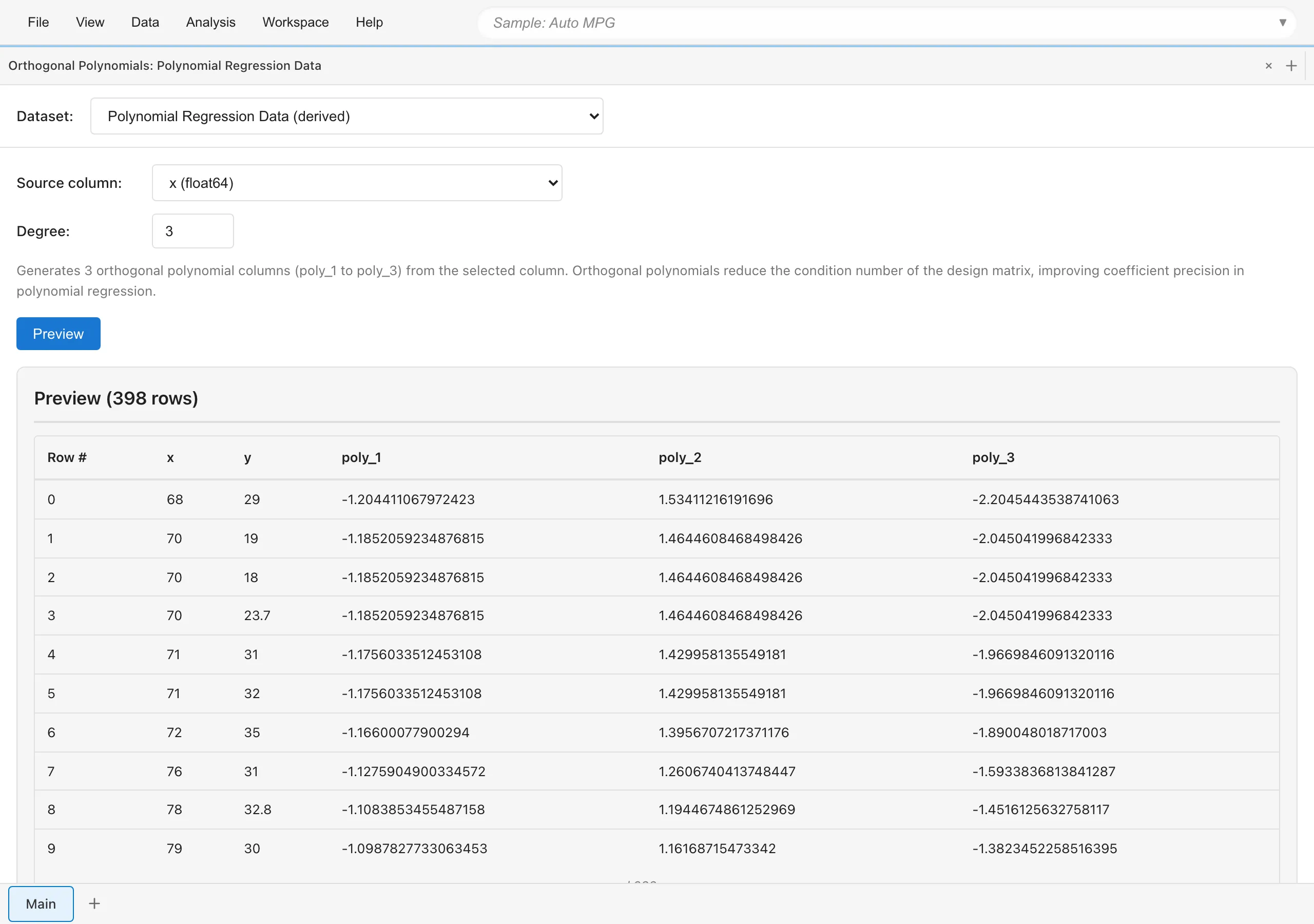
Generating Columns

Select the target dataset from the Dataset dropdown
Select the numeric column to transform in Source column
Set the maximum polynomial degree in Degree (1 to 30). The degree must be less than the number of valid data points in the source column (rows after excluding null, NaN, and Infinity)
Click Preview to inspect the result
Enter a name for the output dataset in Output Name
Click Save as Dataset

The original dataset is not modified. A new derived dataset is created. Rows with null, NaN, or Infinity in the source column are excluded from the derived dataset. For the remaining rows, all original columns are retained and poly_1, poly_2, ..., poly_{degree} columns are appended. The output dataset may have fewer rows than the original.

Each orthogonal polynomial column is normalized so that the sum of squares of its elements equals the number of valid data points $n$ , that is, $\|P_j\|^2 = n$ .

To transform multiple numeric columns into orthogonal polynomials, select the derived dataset you generated from the Dataset dropdown, choose a different Source column, and run again. If columns such as poly_1 already exist, the new columns are named with the source column name appended, such as poly_1_x2.

Generating degree-3 orthogonal polynomials from the x column

Polynomial Regression Workflow

To use orthogonal polynomials instead of the raw polynomial basis:

In the Orthogonal Polynomials tab, generate degree- $d$ polynomial columns from the x column and save the dataset
Open a Linear Regression tab and select the saved derived dataset
Set y as the response variable
Set poly_1, poly_2, ..., poly_d as explanatory variables

R-squared, RMSE, fitted values, and prediction intervals are identical to those from raw polynomial regression. The coefficients are expressed in the orthogonal polynomial basis and differ in both value and interpretation from the raw polynomial basis coefficients. Each poly_j coefficient represents how much the $j$ -th orthogonal polynomial component contributes to the response variable. Because the basis is orthogonal, the coefficient estimates are uncorrelated with each other, and adding higher-degree columns as predictors does not change the lower-degree coefficient estimates. The estimate and confidence interval of the highest-degree poly_d coefficient show the magnitude of the degree- $d$ contribution and the precision of its estimate.

To choose the polynomial degree, run regressions with different degrees and compare AIC or Adj. R-squared in Linear Regression. AIC favors the model with the smaller value; Adj. R-squared favors the larger value. Orthogonal polynomials improve numerical precision but do not prevent overfitting.

Next steps

Linear Regression - Regression analysis with orthogonal polynomial columns