Getting Started

MIDAS is an exploratory data analysis tool that runs in your browser. Your data is processed locally and never sent to external servers (details). No installation required - start analyzing right away.

Tutorial: Exploratory Data Analysis with the Iris Dataset

1. Open Sample Data

This tutorial uses sample data. To use your own CSV file, see Data Preparation and Import.

To start without data, click New Empty Project on the launcher screen. A project with no datasets opens under the name "Untitled Project", showing the Project Overview tab. You can rename the project on the Project Overview tab. Add datasets by entering values with New Dataset... in the Data menu or by generating them with Generate Synthetic Data....

1. Open MIDAS - the launcher screen appears
2. Click Iris dataset from the "Sample Data" section
3. The project screen opens

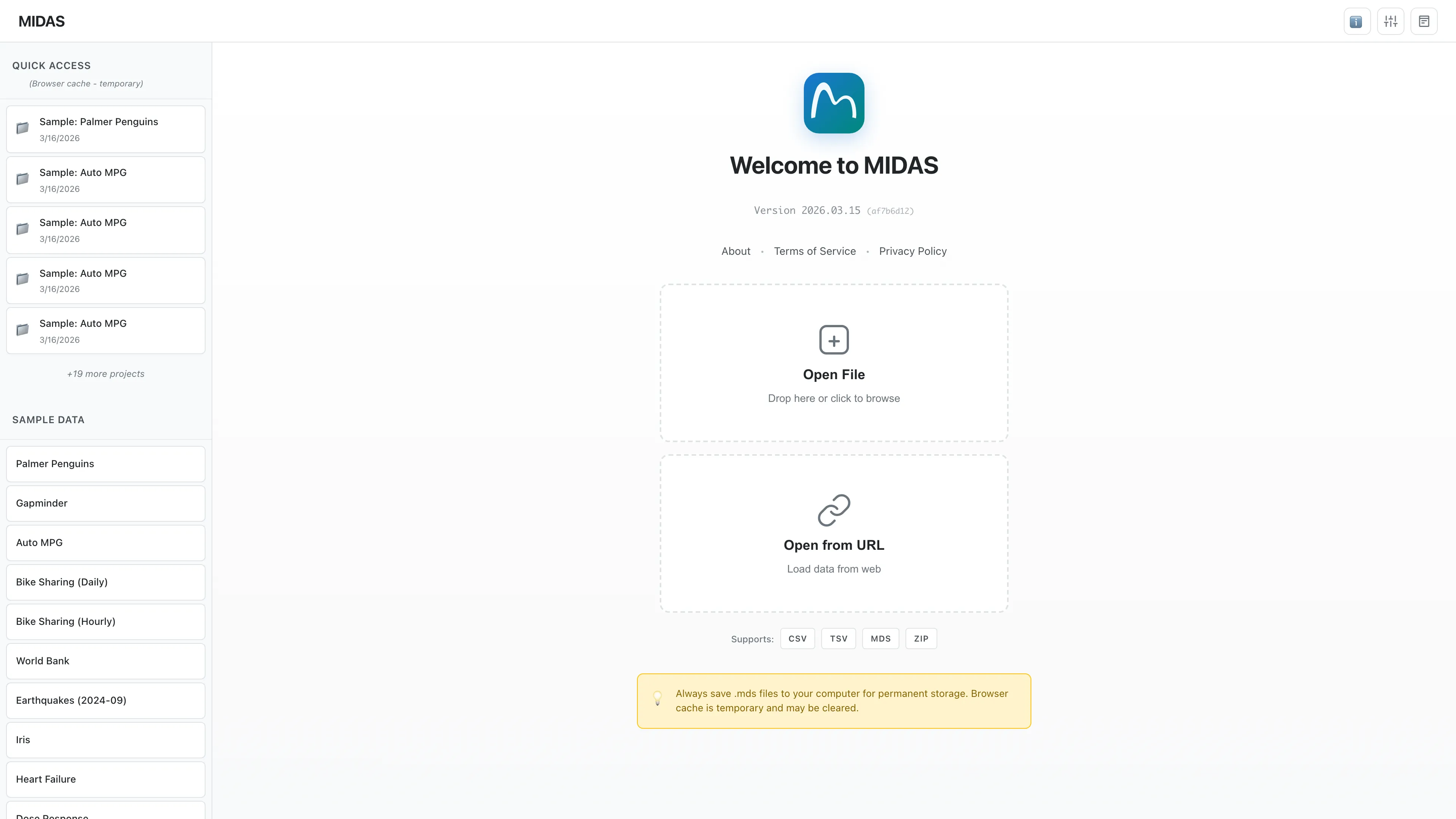
The Iris dataset contains measurements of petals and sepals from three species of iris flowers (150 rows x 5 columns, measurement unit: cm).

2. Explore the Data

The project screen is split into two panes, and three tabs open automatically:

• Data Table (left): Displays data in tabular format
• Statistics (right): Summary and statistics of every column
• Selected Columns (right, the tab next to Statistics): Details of the selected columns

Try the interactive demo below. Click a row in the Statistics tab to expand the details of that column.

Each column header shows the data type (float64, string, etc.) and measurement scale (interval, nominal, etc.). Click the button at the right edge of a column to sort by that column.

MIDAS automatically infers data types and measurement scales when loading data. Loading creates two datasets: Iris (raw), which keeps the original values as text, and Iris, converted to the inferred types. Iris is the one to analyze and opens by default. If the inference is incorrect, right-click a column to change it. Measurement scales affect statistical analysis and graph creation. For example, mean and standard deviation are not calculated for nominal columns. See Data Preparation and Import for details.

3. View Basic Statistics

Let's check basic statistics to understand the data overview.

1. Click a column name in the Data Table tab (e.g., sepal_length)
2. The row for that column expands in the Statistics tab on the right, showing a histogram and statistics

Statistics displayed:

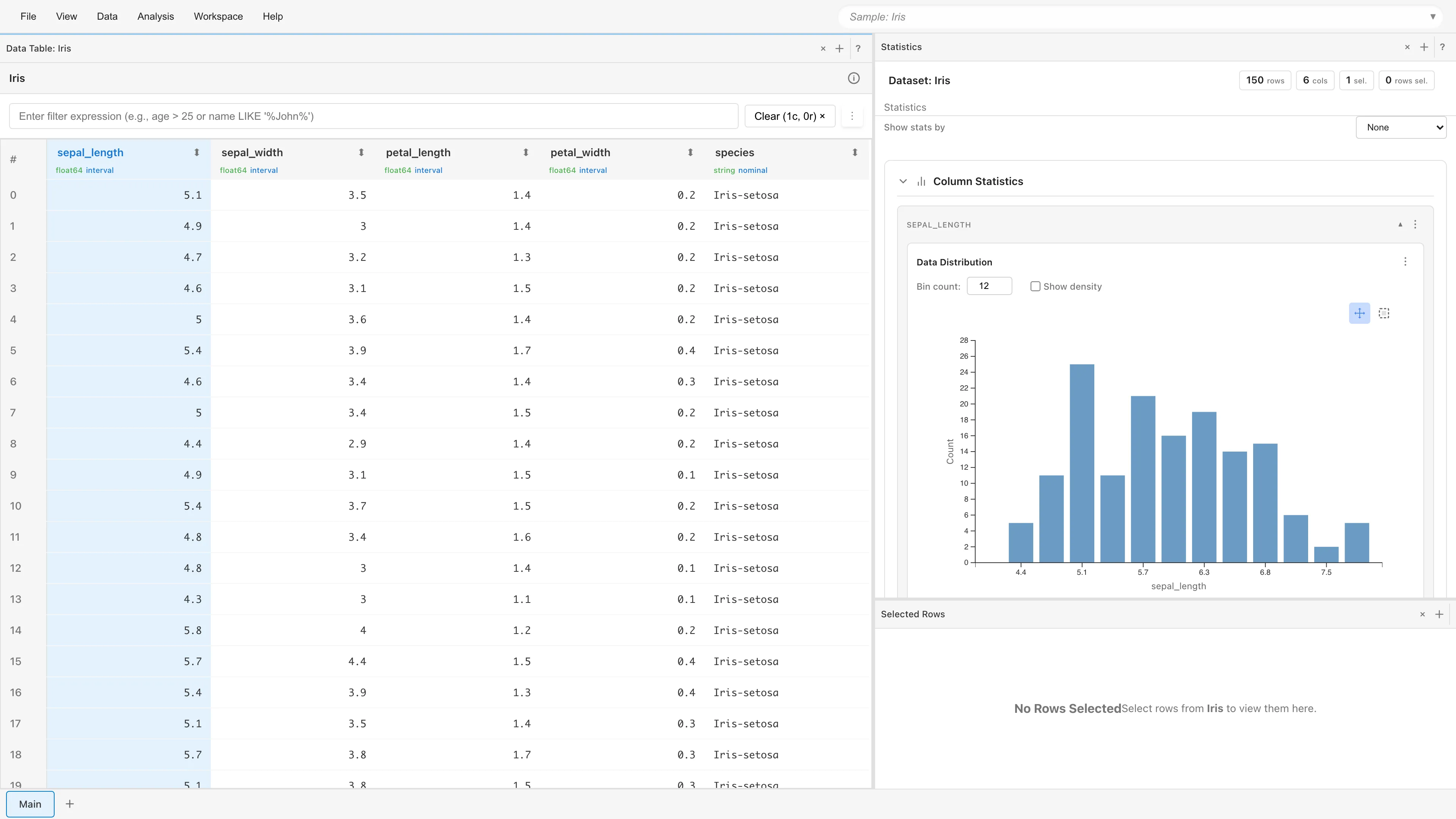
• Moments: mean, std (sample standard deviation), skewness, ex. kurt (excess kurtosis)
• Spread: iqr (interquartile range), range
• Quantiles: 0%(min), 1%, 5%, 10%, 25%, 50%, 75%, 90%, 95%, 99%, 100%(max)

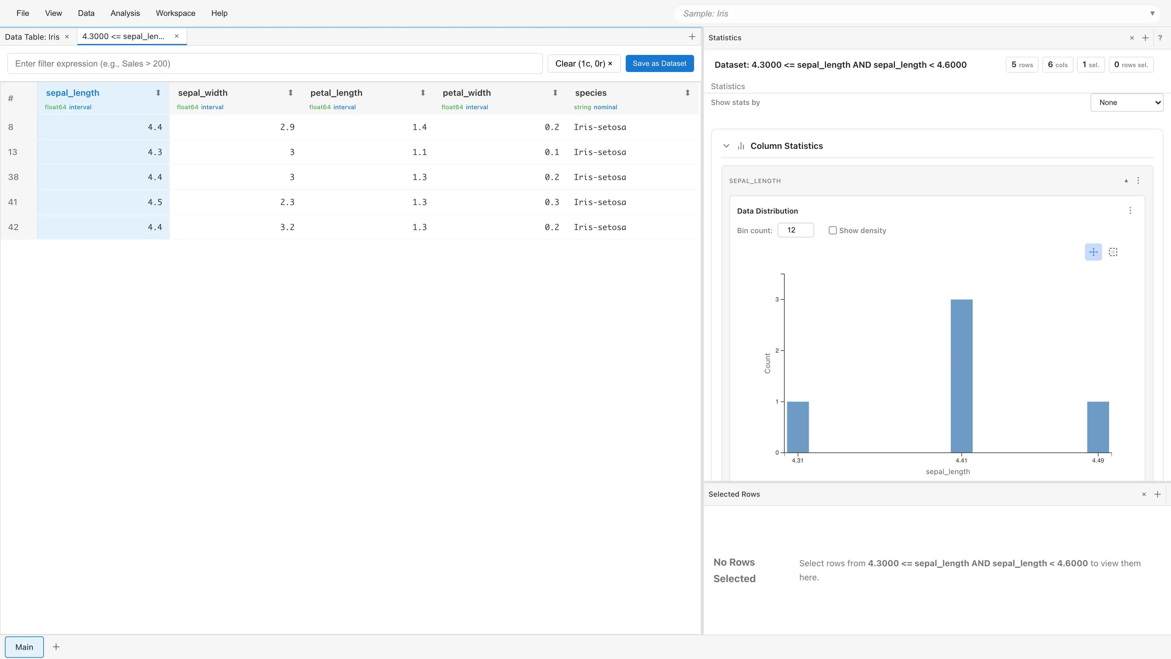
Select rows from histogram:

Click a bar in the histogram to select rows within that range. Selected rows are highlighted in the Data Table.

Double-click a bin to open a new Filtered Data tab containing only the data in that bin. You can view statistics and create graphs from the filtered data. The original dataset is not modified.

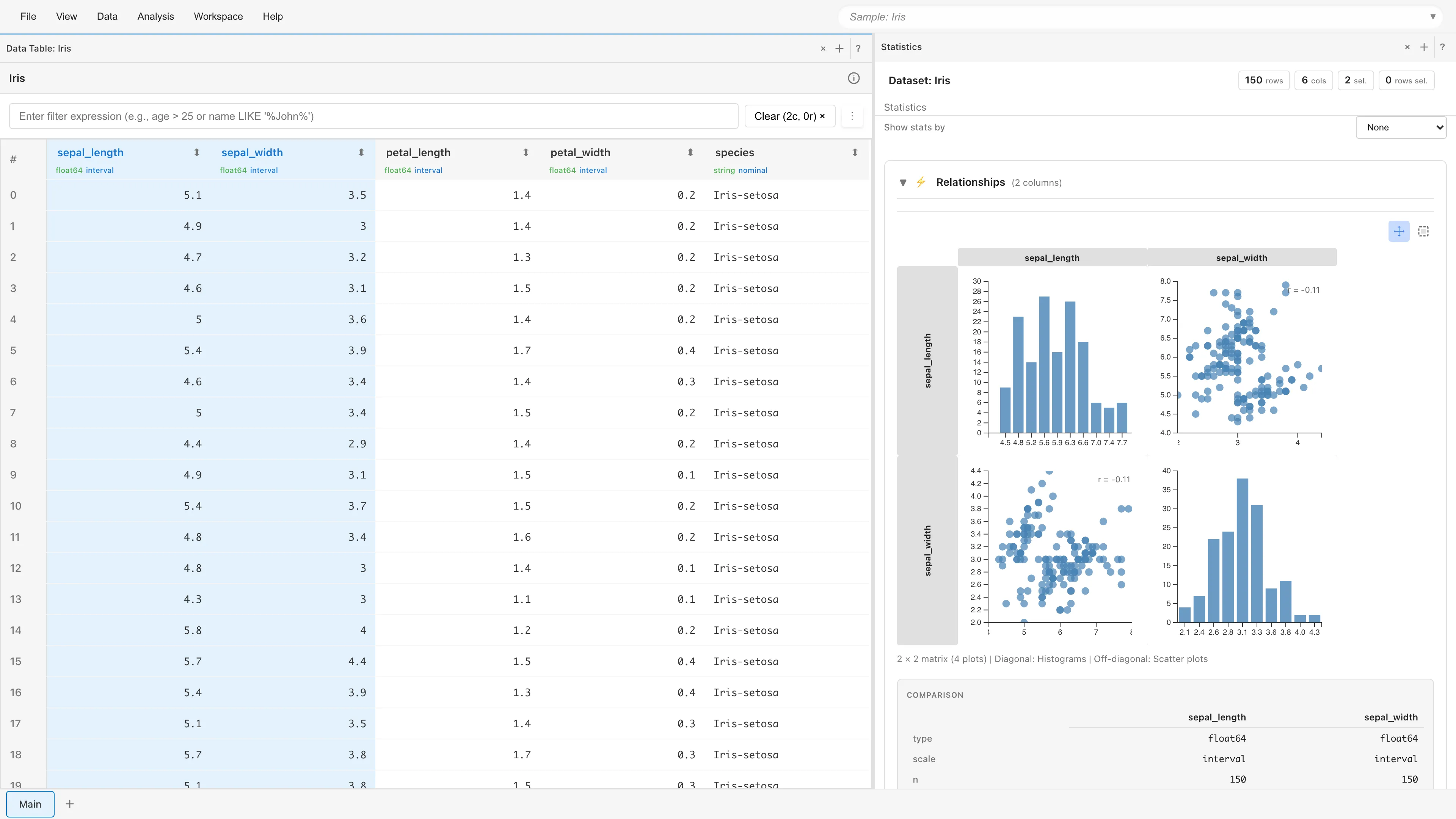
Select two columns to view relationships:

1. With sepal_length selected, Ctrl/Cmd+click sepal_width
2. Switch to the Selected Columns tab on the right to see the statistics and a scatter plot of the two columns

4. Create Graphs

Let's visualize the data to discover patterns.

Create a Scatter Plot

1. Select Analysis → Graph Builder... from the menu bar
2. Select Scatter Plot from Graph Type
3. Select from each dropdown:
   • X-Axis: sepal_length (interval) (sepal length)
   • Y-Axis: sepal_width (interval) (sepal width)
   • Color (Optional): species (nominal) (iris species)
4. A scatter plot appears, color-coded by species

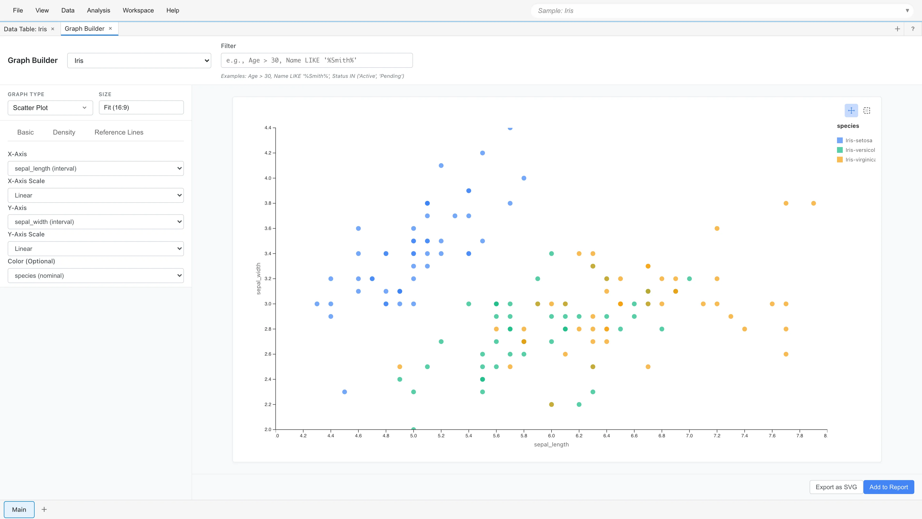
You can compare distribution patterns across species.

See The Graph Builder Tab and Advanced Graph Creation for more details.

5. Save Your Project

MIDAS offers two ways to save your work.

Save to Browser

1. Select File → Save to Browser (or Ctrl/Cmd+S)
2. The project is automatically saved to your browser

Next time you open MIDAS, saved projects appear in the "Quick Access" section of the launcher screen for quick resumption. Clearing browser data will delete saved projects, so export important projects as files too.

Export as File

1. Select File → Export Project... (or Ctrl/Cmd+Shift+S)
2. Confirm or edit the file name (defaults to the project name)
3. The first time you export, enter a signer name (it is included in the signature and shown to recipients)
4. Click Save
5. The project file (.mds format) is downloaded

Exported MDS files can be shared with other users. Files are always digitally signed, so recipients can confirm who created them and detect tampering. See Project Files (MDS) for details.

Open an Exported File

1. In the MIDAS launcher screen, click Open File
2. Select a saved .mds file
3. The project loads and restores to its saved state

Next steps

• The Graph Builder Tab - Create bar charts, scatter plots, pair plots, and more
• Data Preparation and Import - Load your own CSV files
• The Linear Regression Tab - Model data with linear regression

Related Pages

• Project Files (MDS) - Project file format and data privacy
• Sample Datasets - Other sample data included in MIDAS
• Data Types and Measurement Scales - Statistical meaning of measurement scales
• Advanced Graph Creation - Flexible visualization with Grammar of Graphics
• PWA and Offline Use - Install as an app and work offline
• Report - Compile graphs and statistics into a document
• Storage Management - Delete saved projects and check storage usage

Also available as a Markdown file.