Principal Component Analysis (PCA)

The PCA tab performs principal component analysis. PCA summarizes many variables into fewer composite variables (principal components) ordered by how much variance they capture. Use it to explore correlation structures among variables or to reduce dimensionality.

MIDAS computes principal components via eigenvalue decomposition of the covariance matrix.

Basic Usage

Opening PCA

Select Analysis > Principal Component Analysis... from the menu bar to open a new PCA tab.

Setting Up Variables

Variable setup

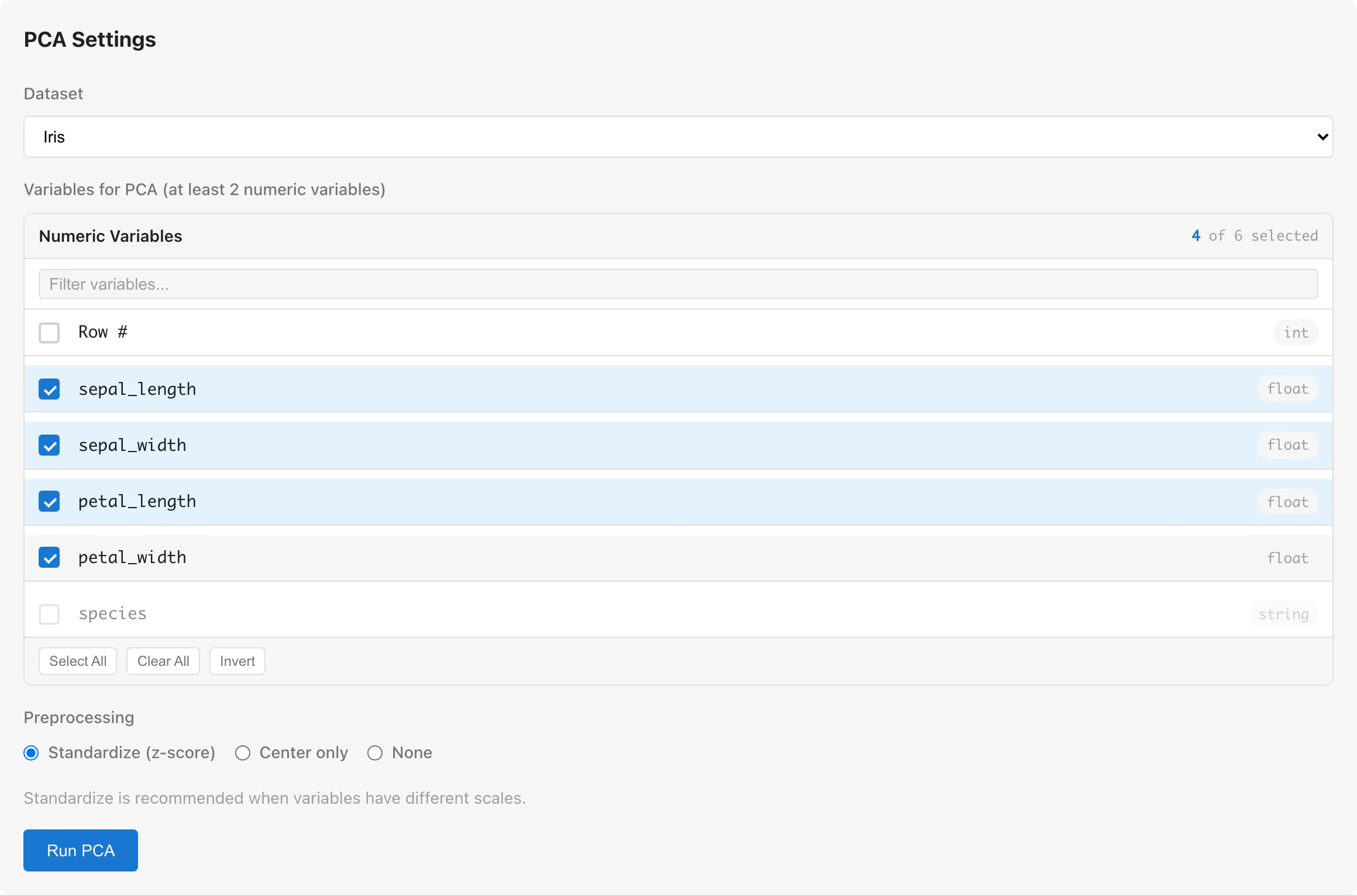
Dataset selects the dataset to analyze.

Variables for PCA selects the variables for the analysis. Only numeric columns are selectable. Columns with nominal/ordinal scale or date/datetime type are grayed out with a tooltip indicating that conversion is required. To use categorical variables, convert them to dummy variables using Dummy Coding first. At least 2 variables are required.

Preprocessing selects the preprocessing method.

Option	Description
Standardize (z-score)	Subtract the mean and divide by the standard deviation for each variable (default)
Center only	Subtract the mean for each variable
None	No variable transformation

Select Standardize when variables have different scales (different units or value ranges). Without standardization, variables with larger ranges dominate the principal components. Center only or None is appropriate when all variables share the same unit and similar scales.

Regardless of the preprocessing choice, the mean is subtracted internally when computing the covariance matrix and principal component scores. With None, variable scales are unchanged but the covariance matrix is computed from mean-centered data. Standardize uses the covariance matrix of standardized data, producing results similar to correlation-matrix-based PCA. Center only and None use the covariance matrix on the original scale.

Click the Run PCA button to run the analysis.

Understanding Results

PCA results

Summary

Displays an overview of the analysis.

Field	Description
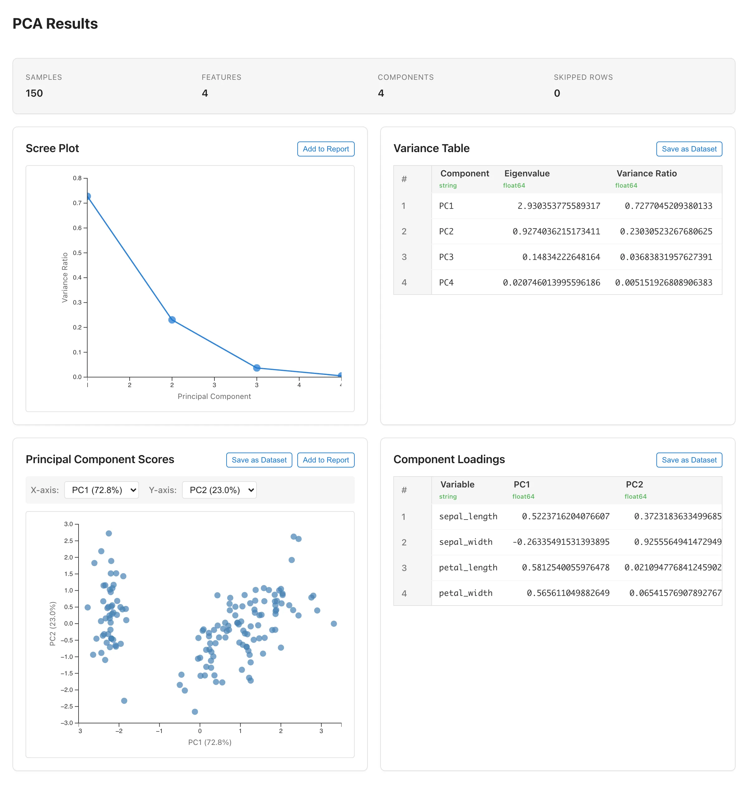
Samples	Number of rows used
Features	Number of selected variables
Components	Number of extracted principal components (equals the number of variables)
Skipped Rows	Rows excluded due to missing or invalid values

Scree Plot

Shows the variance ratio (%) of each principal component as a line chart. The x-axis is the component number and the y-axis is the variance ratio.

The "elbow" — the point where the decline in variance ratio levels off — is one guide for choosing how many components to retain. Use it together with the cumulative variance ratio in the Variance Table. The elbow is a visual judgment and may not always be clear-cut.

Click Add to Report to add the chart to a report.

Variance Table

Displays the eigenvalue and variance ratio for each principal component.

Column	Description
Component	Component number (PC1, PC2, ...)
Eigenvalue	Eigenvalue (amount of variance explained by the component)
Variance Ratio	Proportion of total variance explained (eigenvalue divided by the sum of all eigenvalues)
Cumulative	Cumulative variance ratio

Click Save as Dataset to save as a dataset. The saved dataset opens in a Data Table tab.

Principal Component Scores

Displayed when there are 2 or more components. Plots each observation's principal component scores as a 2D scatter plot.

The X-axis and Y-axis dropdowns switch which components to display. Each option shows the variance ratio (e.g., "PC1 (45.2%)"). The default is X = PC1, Y = PC2.

Click Save as Dataset to save all component scores as a dataset. The saved scores can be used as input data in other analysis tabs (scatter plots, regression, etc.). Click Add to Report to add the chart to a report.

Component Loadings

Displayed when there are 2 or more components. Shows how each variable contributes to each principal component.

Column	Description
Variable	Original variable name
PC1, PC2, ...	Loading on each component

The loadings displayed by MIDAS are eigenvector elements (the weight of each variable in composing the component), not correlations between variables and components. Each eigenvector is normalized to unit length, so individual elements fall between -1 and 1. Variables with larger absolute loadings characterize the component more strongly. The sign indicates a positive or negative relationship with the component.

Click Save as Dataset to save as a dataset.

Notes

Automatic Exclusion of Missing and Invalid Values

Rows containing missing values (null), non-numeric values, or infinities are excluded automatically. The number of excluded rows is shown in the Summary. This exclusion is listwise deletion. With many variables, even a single missing value in any variable causes the entire row to be excluded, potentially reducing the usable sample size substantially. See Missing Data Mechanisms for when listwise deletion is appropriate.

Eigenvector Sign Convention

Eigenvectors have inherent sign ambiguity (if $v$ is an eigenvector, so is $-v$ ). MIDAS resolves this by making the element with the largest absolute value positive for each component.

Number of Components

MIDAS extracts as many components as there are variables. It does not automatically select the number of components. Use the Scree Plot and Variance Table to decide how many components are meaningful for your analysis.