Tutorial: Optimizing Injection Molding Parameters

The Problem

A plastics injection molding line is producing parts that fail tensile strength specifications. The engineering team suspects three process parameters:

• Temperature: resin temperature
• Pressure: injection pressure
• CycleTime: molding cycle time

Changing one parameter at a time only reveals its effect under one fixed combination of the other two, and misses interactions between parameters. A designed experiment that varies all three simultaneously isolates each parameter's contribution with fewer total runs.

Design the Experiment

Select Analysis > DoE Analysis... from the menu bar to open the DoE Analysis tab. Click New Design... in the top-right corner of the tab to open the design wizard.

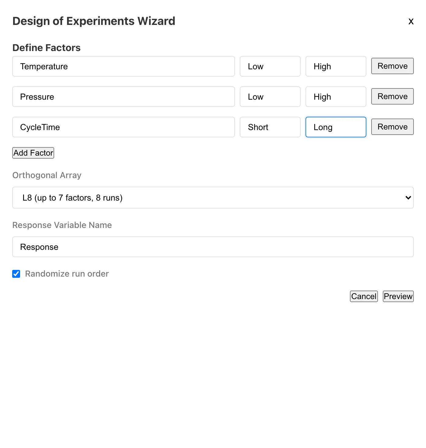
Enter Factors and Levels

Enter the three factors with the two conditions you plan to test:

Factor name	Level 1	Level 2
Temperature	High	Low
Pressure	High	Low
CycleTime	Short	Long

Choose an Array Type

An orthogonal array is an experiment plan table in which factor level combinations are balanced. Every pair of factors has all level combinations appearing equally often, which allows each factor's effect to be estimated independently. The array type determines how many experimental runs you need. The number after L is the run count, and each type has a limit on the number of factors it can handle.

Type	Runs	Max factors
L4	4	3
L8	8	7
L16	16	15

You can use any array type whose maximum is at least your number of factors. A larger array than the minimum gives more data to separate effects from noise.

With 3 factors, all three types are available. L4 needs only 4 runs, but the intercept plus 3 main effects requires 4 parameters against only 4 observations, leaving zero residual degrees of freedom. The error variance cannot be estimated, so neither the precision of effect estimates nor the F-test can be computed. L8 uses 8 runs, which leaves residual degrees of freedom to estimate the error variance and separate real effects from noise.

Set Replications

An orthogonal array specifies one run per condition. Running each condition again with an independent setup provides an estimate of within-condition variability (error). In this tutorial, each condition is run twice for a total of 16 runs. L8 with 1 replication already leaves residual degrees of freedom, but adding replications improves the precision of the error variance estimate.

Set Replications to 2. Each row in the orthogonal array will be duplicated, producing 8 patterns x 2 replications = 16 rows.

Generate the Dataset

Confirm that Randomize run order is enabled. Randomization prevents systematic bias from factors like equipment warm-up or material batch variation that correlate with run order.

Click Preview to inspect the experiment plan. You will see 16 rows: the 8 base conditions from L8, each appearing twice due to the 2 replications. The Response column is empty.

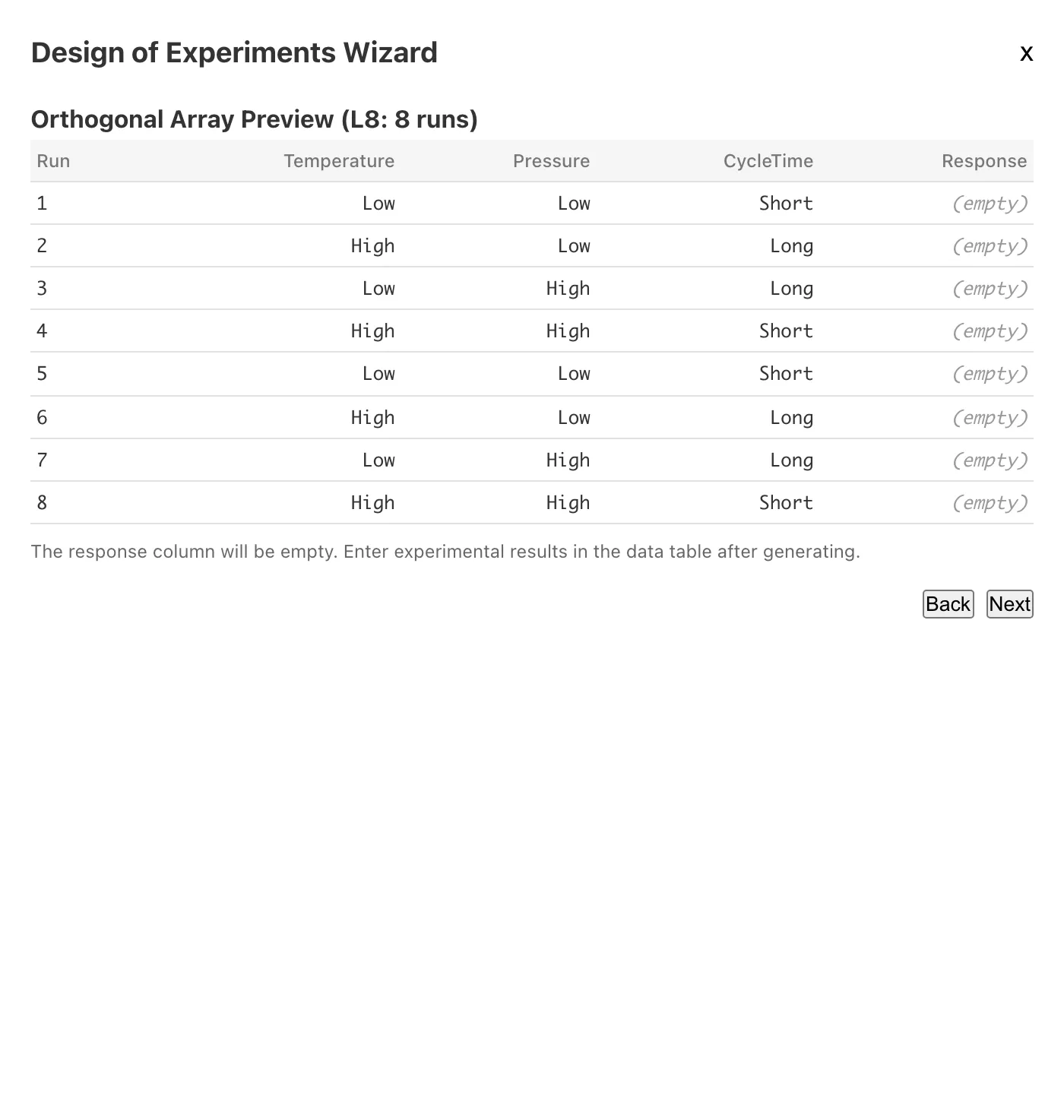
Click Next, confirm the dataset name, then click Generate to add this experiment plan as a dataset in your project.

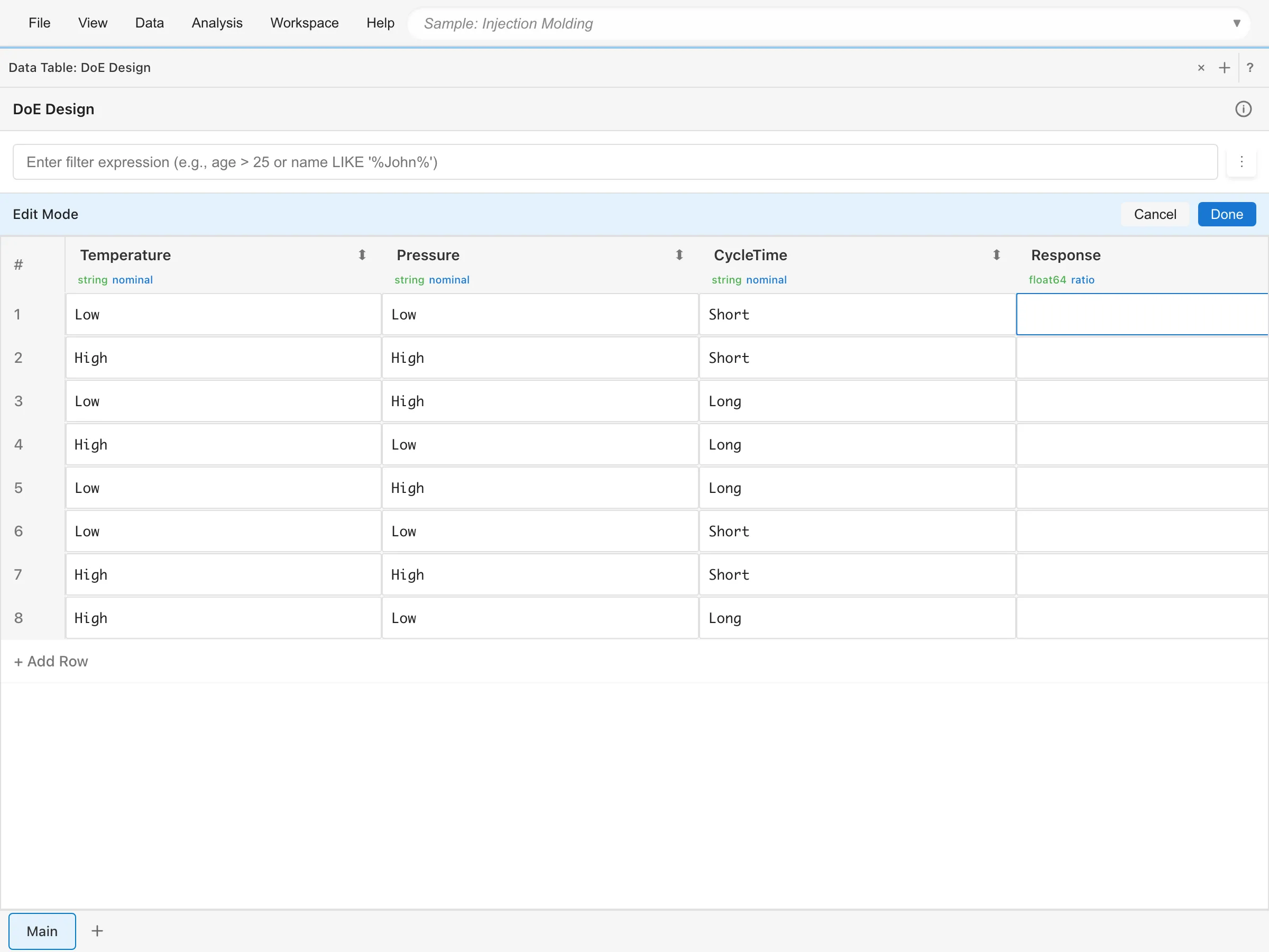
Run the Experiment and Enter Data

The previous steps generated an experiment plan as a dataset. To use your own data, open the dataset in the Data Table tab and double-click cells in the Response column to enter measured strength values.

The rest of this tutorial uses pre-filled sample data to walk through the analysis. Click Injection Molding in the Sample Data section of the launcher. This loads 16 rows: 3 factors x 2 levels x 2 replicates. The sample data rows are sorted by factor levels for readability; in an actual experiment, runs are carried out in randomized order.

Column	Description
Temperature	Resin temperature. High or Low
Pressure	Injection pressure. High or Low
CycleTime	Molding cycle time. Short or Long
Strength	Tensile strength in MPa

Run the Analysis

Select Analysis > DoE Analysis... from the menu bar.

1. Select Injection Molding from Dataset
2. Select Strength for Response Variable
3. Check Temperature, Pressure, and CycleTime under Factors
4. Leave Model set to Main effects only. Start with main effects to understand each factor's contribution, then add interactions if needed
5. Leave Significance Level at the default 0.05

If you select the wrong variable, change the dropdown or checkbox and click Run Analysis again. There is no need to start over.

Click Run Analysis.

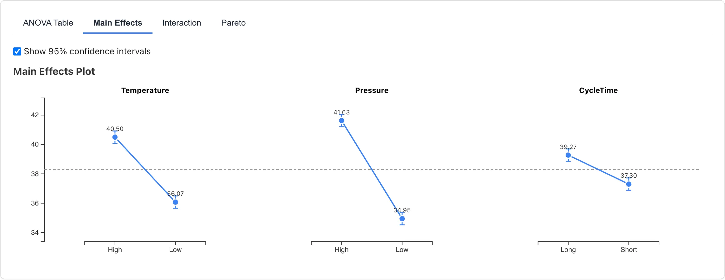
Read the Main Effects Plot

Click the Main Effects sub-tab and check Show 95% confidence intervals.

Each factor's mean strength at each level is shown with confidence intervals. The difference between levels and the width of the intervals show how much each factor affects strength.

• Pressure: Mean 41.63 MPa at High, 34.95 MPa at Low. The difference is about 6.7 MPa, the largest of the three factors
• Temperature: Mean 40.50 MPa at High, 36.08 MPa at Low. The difference is about 4.4 MPa
• CycleTime: Mean 39.28 MPa at Long, 37.30 MPa at Short. The difference is about 2.0 MPa

Confidence intervals show the precision of each level mean estimate. Narrow confidence intervals indicate precise estimation. The horizontal dashed line is the grand mean.

Check for Interactions

Change Model to Main effects + all 2-factor interactions in the settings panel and click Run Analysis. Adding interactions increases the number of parameters and reduces residual degrees of freedom. With this dataset, 7 parameters are estimated from 16 observations, leaving 9 residual degrees of freedom. Without replication, an L8 would leave only 1 residual degree of freedom, drastically reducing the power to detect interactions.

An interaction means that one factor's effect changes depending on the level of another factor. For example, if injection pressure only improves strength when resin temperature is High, then Temperature and Pressure have an interaction. When factors interact, changing one factor alone may not produce the expected result, so you need to find the best combination.

The Interaction sub-tab shows interaction plots. If the two lines in each subplot are roughly parallel, interactions between that factor pair are small. The more the lines cross, the larger the interaction.

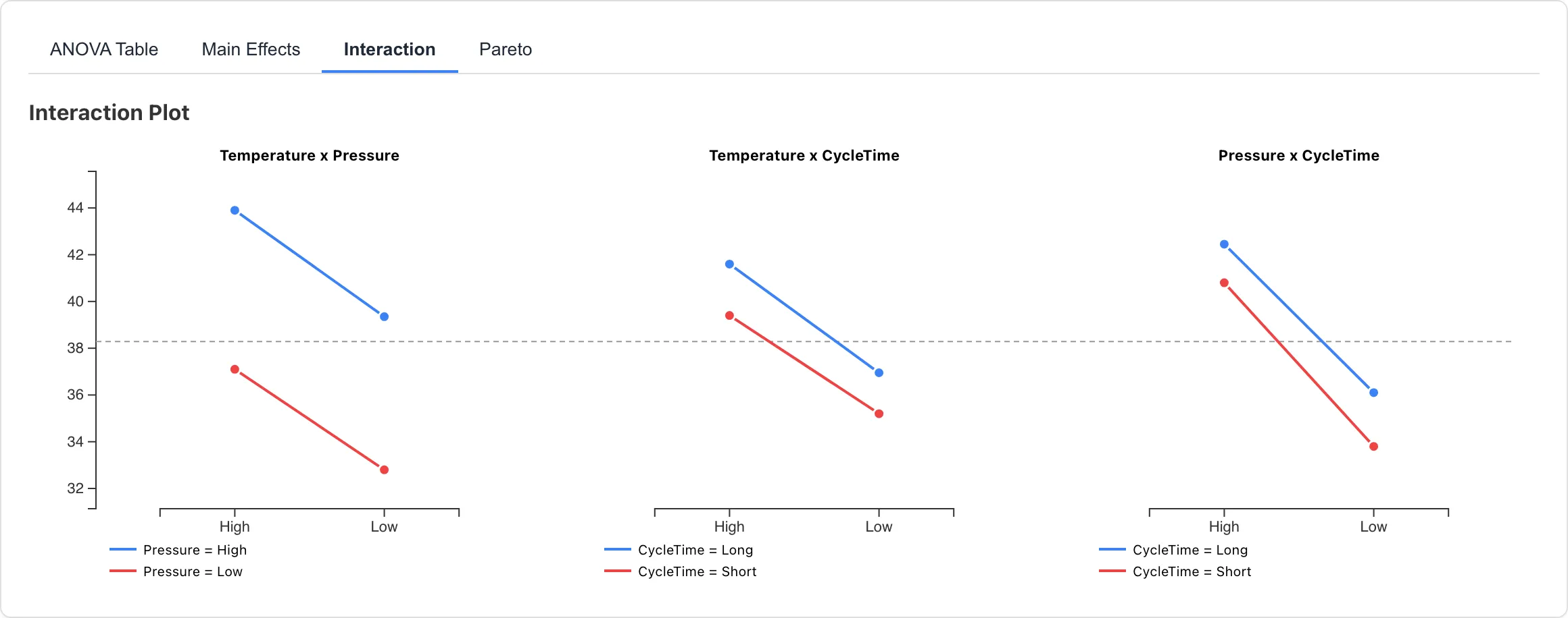
In this dataset, lines are nearly parallel across all three factor pairs. If interactions are large, examine the cell means in the interaction plot and choose the factor combination that yields the best response.

Read the ANOVA Table

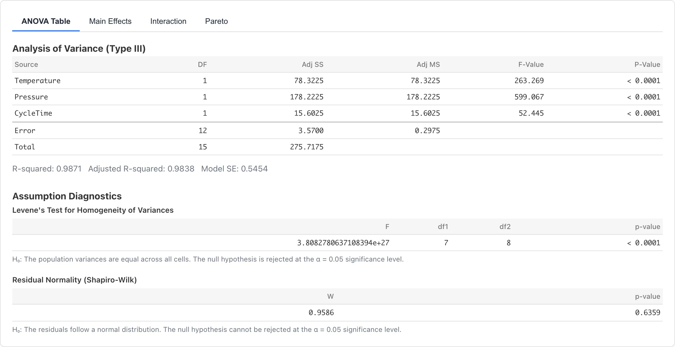
Open the ANOVA Table sub-tab to compare the effect sizes observed in the plots against the F-test results. A P-Value below the significance level of 0.05 indicates that the observed effect cannot be explained by error alone.

In this dataset, all three main effects (Pressure, Temperature, CycleTime) have p-values well below 0.05, confirming that the effects observed in the plots are statistically significant. The interaction terms all have p-values above 0.05, consistent with the nearly parallel lines in the interaction plot.

Make Decisions from the Results

The analysis shows:

• Pressure has the largest effect on Strength: about 6.7 MPa higher at High than Low
• Temperature increases strength by about 4.4 MPa at High, but the effect is smaller than Pressure
• CycleTime has a relatively small effect of about 2.0 MPa
• Interactions between the three factors are small. Each factor's effect is consistent regardless of the other factors' levels

Small interactions mean the three parameters can be optimized independently. Changing Pressure to High is the most effective single action, followed by Temperature. Whether extending CycleTime is worthwhile depends on whether the ~2 MPa gain justifies the longer cycle.

This experiment used randomized assignment of conditions, so the estimated effects support a causal interpretation within these experimental conditions. The effects are specific to the materials, equipment, and factor levels used in this experiment. A typical next step is a confirmation run at Pressure = High, Temperature = High, CycleTime = Long to verify that the same improvement holds under actual production conditions.

Related Pages

• DoE Analysis -- Detailed usage and statistical model documentation
• ANOVA -- One-way and two-way analysis of variance