Random Forest

The Random Forest tab trains and predicts with Random Forest models for classification and regression tasks. Random Forest is an ensemble method that builds multiple decision trees from bootstrap samples and aggregates their predictions (Breiman, 2001) — majority vote for classification, averaging for regression. It does not assume a distribution for the response variable, so there is no need to choose a distribution family or link function as in GLM.

Basic Usage

Opening Random Forest

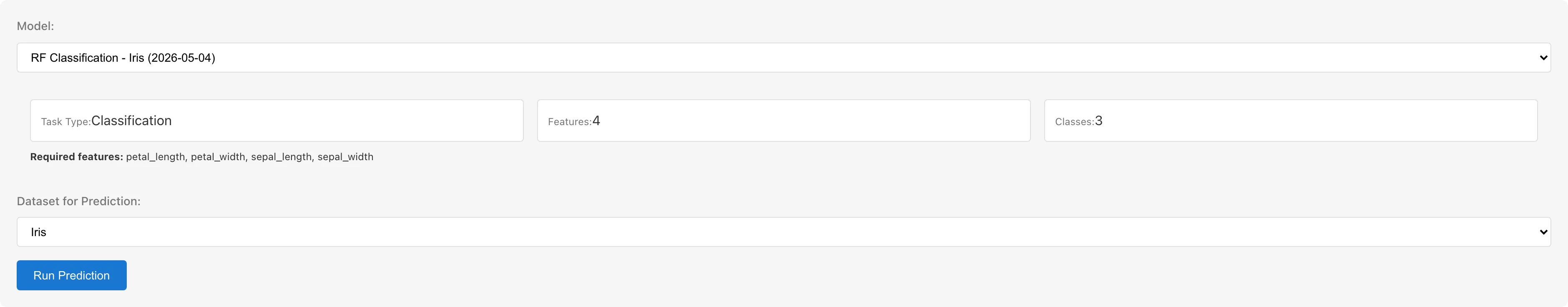
Select Analysis > Random Forest... from the menu bar. The Train and Predict buttons at the top of the tab switch between training and prediction modes.

Setting Up Variables

The examples below use the Iris dataset.

Dataset selects the dataset to analyze.

Task Type selects the type of task.

• Classification: treats target variable values as class labels. All column types are selectable
• Regression: treats the target variable as a continuous value. Only numeric columns (int64, float64) are selectable

Target Variable (Y) selects the response variable. In Regression mode, non-numeric columns are shown as "(requires conversion)" and cannot be selected.

Predictor Variables (X) selects predictor variables. Multiple numeric columns can be selected. Columns with categorical scales (nominal/ordinal) or date/datetime types are not selectable — convert them to numeric dummy variables using the Dummy Coding tab first. The column selected as the target variable is automatically excluded from the candidates.

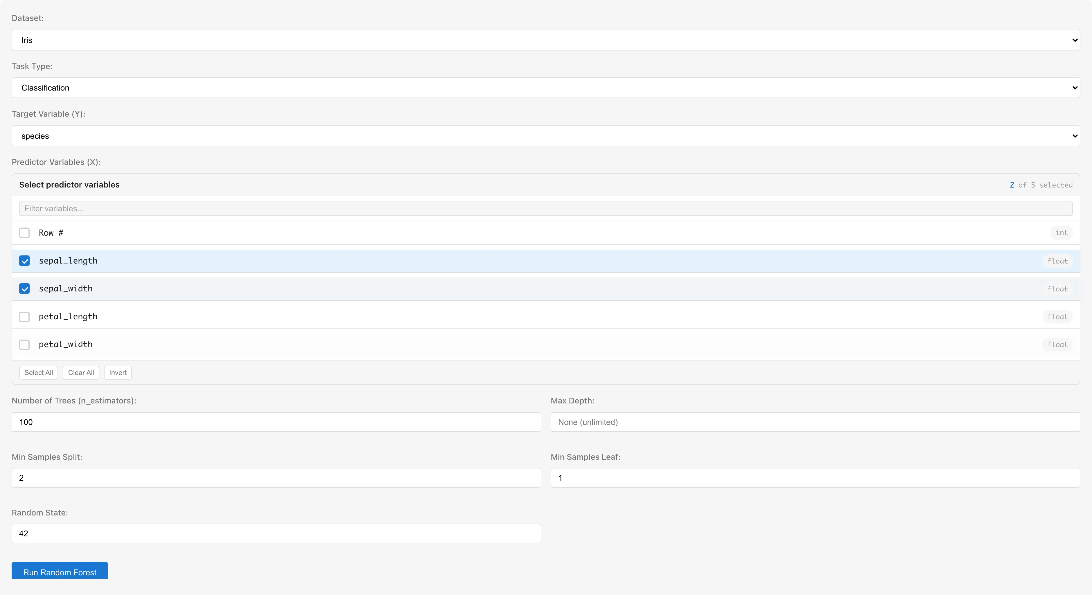
Hyperparameters

Parameter	UI Label	Default	Description
nEstimators	Number of Trees (n_estimators)	100	Number of decision trees in the ensemble
maxDepth	Max Depth	Empty (unlimited)	Maximum depth of each tree. Shallower trees reduce overfitting
minSamplesSplit	Min Samples Split	2	Minimum number of samples required to split an internal node
minSamplesLeaf	Min Samples Leaf	1	Minimum number of samples required in a leaf node
randomState	Random State	42	Random seed. The same value produces the same results

The number of predictors considered at each split is fixed at $\lfloor\sqrt{p}\rfloor$ for both classification and regression, where $p$ is the total number of predictors. Some implementations use $p/3$ for regression, but MIDAS uses $\sqrt{p}$.

Running the Analysis

Click the Run Random Forest button. A progress message is displayed during training.

Understanding Results

Classification Metrics

Shown when Task Type is Classification.

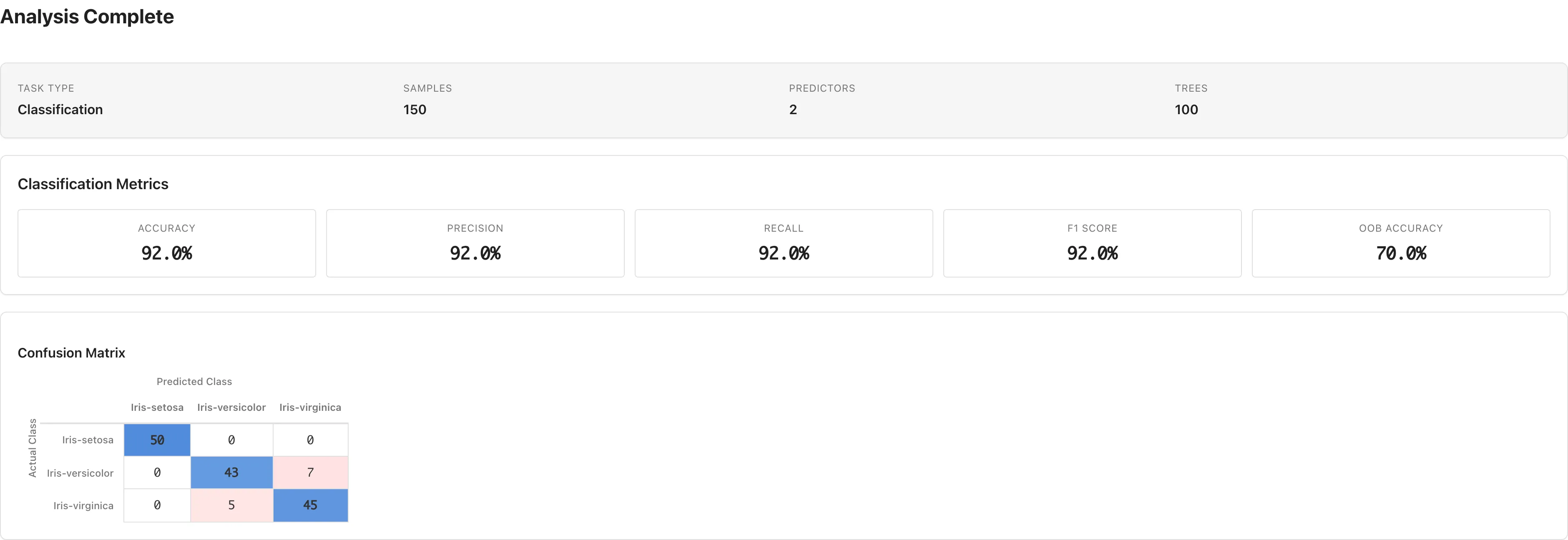
Metric	Description
Accuracy	Proportion of correctly classified samples
Precision	Proportion of true positives among predicted positives
Recall	Proportion of true positives among actual positives
F1 Score	Harmonic mean of Precision and Recall
OOB Accuracy	Out-of-Bag accuracy (see OOB Score)

For binary classification, Precision, Recall, and F1 Score are reported for the second class in the confusion matrix column order. For three or more classes, they are weighted averages using class sample counts as weights.

Accuracy and other metrics above are computed on the training data, so even an overfitting model can show high values. Use OOB Accuracy to judge generalization performance. For binary classification, verify that Precision, Recall, and F1 Score correspond to the intended class by checking the column order in the confusion matrix.

Confusion Matrix

The confusion matrix is displayed below the classification metrics. Rows represent actual classes and columns represent predicted classes. Diagonal elements are the counts of correct classifications.

Regression Metrics

Shown when Task Type is Regression.

Metric	Formula	Description
R-squared ($R^2$)	$1 - \frac{\sum(y_i - \hat{y}_i)^2}{\sum(y_i - \bar{y})^2}$	Proportion of variance in the target explained by the model
RMSE	$\sqrt{\frac{1}{n}\sum(y_i - \hat{y}_i)^2}$	Root mean squared error
MAE	$\frac{1}{n}\sum\lvert y_i - \hat{y}_i\rvert$	Mean absolute error
MSE	$\frac{1}{n}\sum(y_i - \hat{y}_i)^2$	Mean squared error
OOB $R^2$	—	Out-of-Bag $R^2$ (see OOB Score). Negative when the model predicts worse than the mean

R², RMSE, and other metrics above are computed on the training data, so even an overfitting model can show high values. Use OOB $R^2$ to judge generalization performance.

Diagnostic Plots (Regression)

Two scatter plots are displayed in Regression mode. These plots are based on training data predictions and residuals.

Actual vs Predicted: plots actual values ($y$) on the vertical axis against predicted values ($\hat{y}$) on the horizontal axis. Points clustered near the diagonal indicate predictions close to the actual values.

Residuals vs Fitted Values: plots residuals ($y - \hat{y}$) against predicted values. A dashed line at zero is shown. Random Forest fits training data closely, so residuals tend to be small and this plot alone cannot detect overfitting. Use OOB $R^2$ to judge generalization performance.

Clicking or rectangle-selecting data points on either plot shows details (Row, Actual, Predicted, Residual) in a table below.

Feature Importances

Shown for both classification and regression. A sorted table with bar chart visualization displays each predictor's importance.

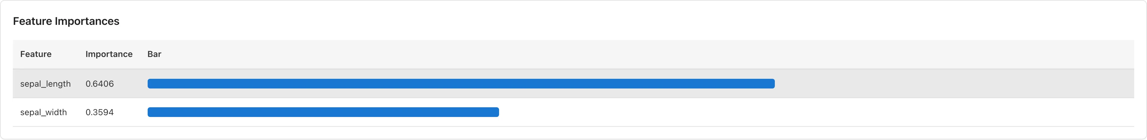
Importance is computed as Mean Decrease in Impurity (MDI). For each predictor, the total reduction in impurity across all trees is summed and normalized to total 1. Gini impurity is used for classification; variance is used for regression.

MDI reflects how often a predictor is used for splits in the training data, so continuous variables with many unique values tend to score higher simply because they offer more split candidates. Conversely, expanding a categorical variable via Dummy Coding spreads its importance across multiple dummy columns, making it appear less important.

Saving the Model

Enter a name in the Model Name field below the results. The default format is "RF Classification - {dataset name} ({date})" or "RF Regression - {dataset name} ({date})".

Click Save Model to save the model to the project. Saved models can be used in Predict mode.

Prediction

Running Predictions

1. Click the Predict button at the top of the tab to switch to prediction mode
2. Select a saved model from the Model dropdown. Model information (Task Type, number of predictors, required predictor names, number of classes for classification) is displayed
3. Select a dataset from Dataset for Prediction. The dataset must contain columns matching the model's predictor names
4. Click Run Prediction

Prediction Results

After prediction completes, the following are displayed.

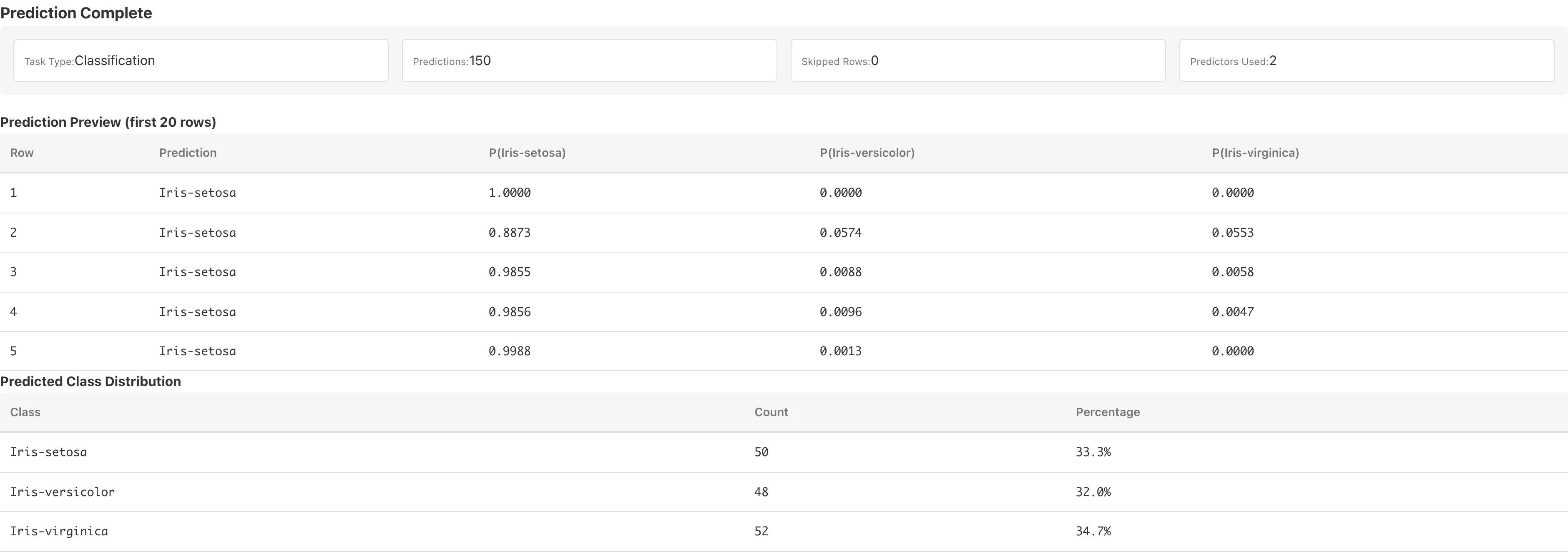
Preview table: the first 20 rows of predictions. For classification, predicted probabilities P(class name) for each class are also shown.

Predicted Class Distribution (classification only): counts and percentages for each predicted class.

Prediction Statistics (regression only): summary statistics of predicted values (Mean, Median, Std Dev, Min, Max).

Save as Dataset

Click Save as Dataset to save the predictions as a derived dataset.

Column	Content
Predictor columns	Columns from the source dataset matching the model's predictors
Prediction	Predicted value. Class label (string) for classification, numeric value (float64) for regression
P(class name)	Predicted probability for each class (classification only, float64)

Rows with missing predictor values have null in the prediction columns.

Notes

Using Categorical Variables

Only numeric variables can be used as predictors. To use categorical variables, convert them to numeric dummy variables using the Dummy Coding tab before running the analysis.

Automatic Exclusion of Missing Values

During training, rows containing missing values (null), non-numeric values, or infinity in the selected variables are automatically excluded. When exclusions occur, the Samples field in the results shows the number of excluded rows. This is listwise deletion. See Missing Data Mechanisms for conditions under which it yields valid estimates.

During prediction, rows with missing predictor values are skipped and receive null in the prediction columns. The number of skipped rows is reported in the results.

Out-of-Bag (OOB) Score

Each tree is trained on a bootstrap sample (sampling with replacement, same size as the original data). The OOB score is computed by predicting each training sample using only the trees whose bootstrap samples did not include that sample. Accuracy is shown for classification; $R^2$ for regression.

Each bootstrap sample includes about 63.2% of the data; the remaining ~36.8% ($1 - (1 - 1/n)^n$) serve as the OOB validation set. This provides a generalization estimate without a separate holdout.

Limitations

• Random Forest training runs in JavaScript within the browser. Large datasets or high numbers of trees may take noticeable time
• Cross-validation and train/test splitting are not available; the OOB score serves as the generalization estimate
• The number of predictors considered at each split (maxFeatures) is fixed at $\lfloor\sqrt{p}\rfloor$ and cannot be changed from the UI

References

• Breiman, L. (2001). Random Forests. Machine Learning, 45(1), 5–32. https://doi.org/10.1023/A:1010933404324

See Also

• Linear Regression — parametric linear models
• Generalized Linear Model (GLM) — regression with distributional assumptions
• Dummy Coding — convert categorical variables to numeric