The ANOVA Tab

The ANOVA tab analyzes whether the means of a response variable differ across groups defined by categorical variables. Both one-way and two-way designs are supported. It assumes independent, between-subjects observations and does not support repeated measures or paired data—for example, the same patient measured before and after treatment or multiple samples from the same unit. For those designs, use a GLMM with the subject as the random-effect group.

Basic Usage

Open the Tab

Select Analysis > ANOVA... from the menu bar.

Run an Analysis

Configure the following in the settings panel:

1. Select a dataset from Dataset
2. Choose One-Way or Two-Way under Analysis Type
3. Select a categorical variable for Factor A (Categorical)
4. Select a numeric variable for Response Variable (Numeric)
5. Click Run Analysis

Data Format

Data must be in long format with one row per observation. Each row contains the factor value and the response variable value. Use Reshape to convert wide-format data.

One-Way ANOVA

Analyzes differences in the response variable means across groups defined by a single categorical factor. Use this when you have one grouping factor.

Statistical Model

$y_{ij} = \mu + \alpha_i + \varepsilon_{ij}$

$y_{ij}$ is the $j$-th observation in group $i$, $\mu$ is the overall mean, $\alpha_i$ is the effect of group $i$, and $\varepsilon_{ij}$ is the error term.

Assessing Group Differences

ANOVA decomposes the total variation in the response variable into between-group variation and residual variation. The decomposition appears as SS, df, and MS in the ANOVA table. Of the effect sizes, η² shows the proportion of the total variation attributable to the factor in the sample, and ω² is an estimate of that proportion in the population. The magnitude and precision of group differences can be read from the simultaneous confidence intervals for pairwise differences from Tukey HSD. The group mean confidence intervals in Group Statistics show the precision of each group mean estimate.

Variable Selection

Which columns can be selected as factors and as the response variable follows the column's measurement scale. Columns that do not meet the requirement still appear in the list, but are grayed out and cannot be selected. A short reason is appended after the column name.

Factor A (Categorical) and Factor B (Categorical) take a categorical variable that defines the groups. Columns with a nominal or ordinal scale can be selected. When an ordinal column is selected, ANOVA estimates no ordered contrast such as a linear trend and groups the levels the same way it groups a nominal column. For an enum column, the order of the enum definition sets the row order in Group Statistics and the direction of the Tukey HSD differences. That order comes from the enum definition, not from the measurement scale.

A numeric column that encodes categories, such as a dose code or a batch number, can also be used as a factor. Right-click the column header in Data Table and change its scale to nominal or ordinal from Edit Scale of Measurement. Each distinct value of the column then forms one group, and the groups are ordered as text, so 10 comes before 2. Do not do this with a measured quantity. Nearly every value would form a group of its own, leaving no degrees of freedom for the residuals.

Response Variable (Numeric) takes the numeric variable to analyze. Columns with an interval or ratio scale can be selected. The measurement scale is a declaration about the column, and ANOVA does not inspect the values. A column whose scale says interval but whose cells hold text appears as an option, and rows that cannot be converted to numbers are dropped as invalid values.

A boolean column has a nominal scale by default and therefore cannot be selected as it is. Changing its scale to ratio makes it selectable, and its values are read as 0 and 1. In a 0/1 response the variance within a group is determined by that group's mean, so groups with different proportions do not have equal variances. Intervals computed from the pooled MSE can fall outside 0 and 1. To work with proportions, use a GLM with the binomial family.

Date and datetime columns cannot be used as the response variable even though their scale is interval. To analyze an elapsed duration, build a numeric column of days from a baseline date in the SQL Editor and select that column.

The measurement scale belongs to the column itself, so changing it here also affects graph axis types and the options offered by the other analysis tabs.

When a selected column stops meeting the requirement, the settings panel shows the reason and Run Analysis becomes unavailable. Reloading the dataset or changing the column's scale can produce this state, as can pointing Factor A and Factor B at the same column in a two-way design. Select another column, or restore the scale of that column.

Example

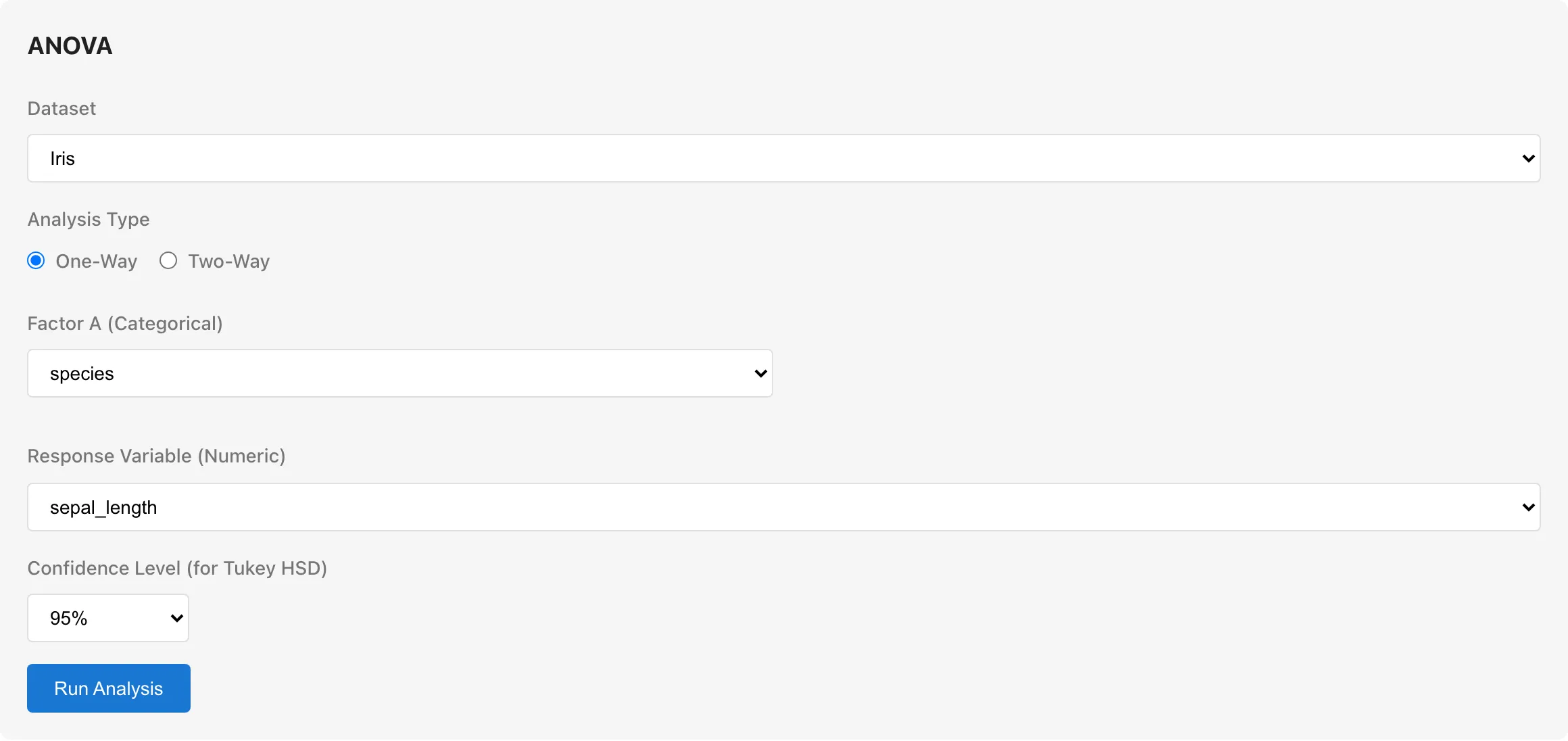
To analyze whether sepal length differs among the three species Iris-setosa, Iris-versicolor, and Iris-virginica in the Iris sample data:

1. Dataset: Iris
2. Analysis Type: One-Way
3. Factor A: species
4. Response Variable: sepal_length
5. Click Run Analysis

Confidence Level

Set the confidence level for Group Statistics confidence intervals and Tukey HSD post-hoc comparisons. Choose from 90%, 95% (default), or 99%. The Tukey HSD confidence interval width matches the confidence level. This setting also appears in two-way ANOVA, where it applies to the Group Statistics confidence intervals.

Two-Way ANOVA

Analyzes the effects of two categorical factors and their interaction on the response variable. Use this when you have two grouping factors.

Statistical Model

With interaction:

$y_{ijk} = \mu + \alpha_i + \beta_j + (\alpha\beta)_{ij} + \varepsilon_{ijk}$

$\alpha_i$ is the effect of factor A, $\beta_j$ is the effect of factor B, and $(\alpha\beta)_{ij}$ is the interaction effect.

Additional Settings

Factor B (Categorical): Select a second categorical variable, different from Factor A.

Include interaction term (A x B): Whether to include the interaction term in the model. Enabled by default. Include the interaction when the effect of one factor may depend on the level of the other. If the interaction is known to be absent, excluding it increases the residual degrees of freedom, providing a more precise estimate of the error variance.

Sum of Squares Type: Choose the method for computing sums of squares.

Sum of Squares Types

Type I computes sums of squares sequentially based on the order factors enter the model. Each factor's contribution depends on which factors are already in the model. MIDAS enters Factor A first, then Factor B, then the interaction term. The SS for Factor A is the reduction in residual sum of squares when Factor A is added to the intercept-only model, and the SS for Factor B is the further reduction when Factor B is added. Swapping the Factor A and Factor B assignments changes the results.

Type III computes sums of squares for each factor as if it were the last one entered. Each factor's contribution is adjusted for all other factors.

For balanced designs (equal sample sizes in all cells), Type I and Type III produce identical results. For unbalanced designs, Type III is generally preferred because results do not depend on factor ordering. The default is Type III. Type I is useful when the order of factor entry is meaningful—for example, when adjusting for a covariate before assessing a treatment factor.

Type III Interpretation with Interaction

MIDAS uses treatment coding. Treatment coding designates one level of each factor as the reference category (baseline level) and expresses the effects of all other levels as differences from it. The reference category is the first level in alphabetical order. When the interaction term is included, the Type III main effect for each factor depends on the treatment coding reference category. For example, if Factor A has levels A, B, C and Factor B has levels X, Y, the reference categories are A and X (the first level in alphabetical order). The Type III sum of squares for Factor A represents the additional explanatory power of Factor A's levels compared to a model without them, evaluated when Factor B is at reference level X. With balanced data, this coincides with the effect averaged across all levels of Factor B. With unbalanced data, the two may differ.

Reading the Results

Observations

The total number of observations used in the analysis appears at the top. If rows were excluded, the count of excluded rows is also shown.

Group Statistics

A summary table of descriptive statistics for each group.

Some excluded rows do not appear in the Excluded column: rows with a missing factor value belong to no group, and rows of a level or cell removed entirely by exclusion have no row in the table. When such rows exist, their counts appear as notes below the table.

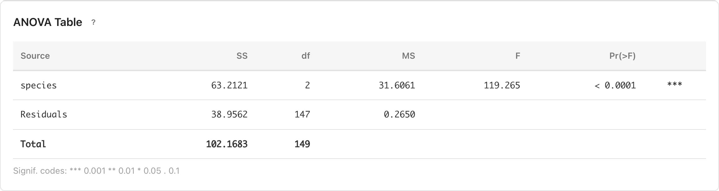
ANOVA Table

The main results table. Decomposes the total variance of the response variable into contributions from each factor and residual error. This table evaluates the magnitude of group differences using effect sizes (η² and ω²). It does not display test statistics (F-values) or p-values. The magnitude and precision of each pairwise difference can be assessed from the simultaneous confidence intervals in Tukey HSD.

When the variation in the response is below floating-point precision relative to its magnitude, the sum-of-squares decomposition is meaningless. This covers responses whose values are all identical, as well as responses with a tiny relative spread on top of a large offset. SS, MS, η², ω², and the Total sum of squares are then undefined and shown as "-", and a warning explains why.

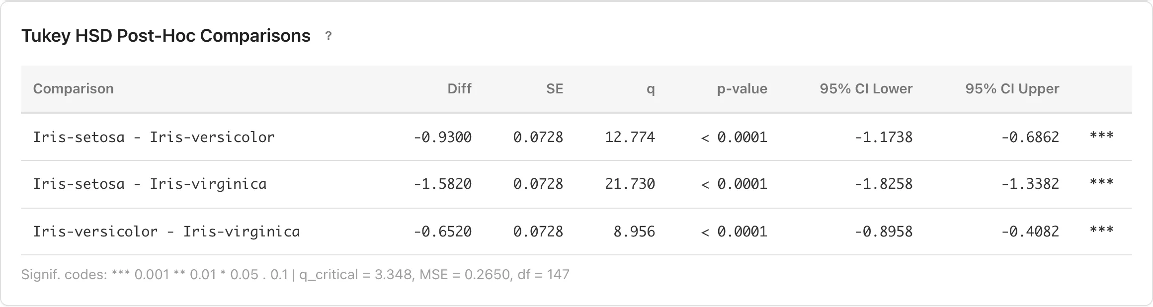
Tukey HSD Post-Hoc Comparisons

The ANOVA table decomposes overall variation among groups, but does not show how large the difference is for each pair. Tukey HSD post-hoc comparisons estimate the mean difference and its simultaneous confidence interval for every pair of groups, allowing you to assess the magnitude and precision of each pairwise difference.

For one-way ANOVA, Tukey HSD is computed automatically. The Tukey-Kramer method is used, which handles unequal group sizes. Tukey HSD is not available for two-way ANOVA.

Tukey HSD constructs simultaneous confidence intervals for all pairwise mean differences. It controls the family-wise error rate, reducing the inflation of false positives compared to running individual t-tests for each pair.

The interval center (the Diff value) is the point estimate of the difference, and the interval width reflects estimation uncertainty. Read the point estimate for the magnitude of the difference and the interval width for how precisely it is estimated.

Tukey HSD uses the pooled MSE, so it assumes equal population variances. When group variances differ substantially, the actual coverage of these intervals may deviate from the nominal level. Compare the group standard deviations in Group Statistics to check this assumption.

The critical value $q_{\text{critical}}$, MSE, and residual degrees of freedom are displayed below the table.

Assumptions

ANOVA assumes the following. Verify that these are reasonable when interpreting results.

• Independence: Observations are independent of each other
• Normality: The response variable follows a normal distribution within each group
• Homogeneity of variance: The variance is equal across all groups

Assumption Diagnostics

ANOVA assumes normality within each group. Two types of Q-Q plots help assess this assumption.

The pooled residual Q-Q plot compares all residuals against a theoretical normal distribution. Points falling close to the diagonal line suggest approximate normality. Departures such as heavy tails or skewness are visible in the shape of the deviation from the line. Because this plot combines residuals from all groups, it can mask departures that affect only some groups.

The per-group Q-Q plots show the residual distribution within each group separately. These provide a visual check of the normality assumption, since ANOVA assumes normality within each group. When there are more than 12 groups, only the first 12 (in the same order as the Group Statistics table) are displayed.

When homogeneity of variance holds, the estimates of group mean differences and their confidence intervals become robust to departures from normality as sample sizes increase. If Q-Q plots show departures from normality, check homogeneity of variance first.

Homogeneity of variance can be assessed by comparing the SD values in the Group Statistics table. When group SDs are similar, minor departures from normality are tolerable. When SDs differ substantially across groups, this robustness does not hold. Consider using GLM, which can explicitly model the variance structure.

In two-way ANOVA, residuals are computed from the fitted values of the selected model. When the interaction term is included, the model fits a separate mean for each cell, so residuals equal deviations from cell means. When the interaction term is excluded, the main-effects-only model produces different fitted values, and the residuals reflect deviations from those predictions. The choice of model affects both the pooled and per-group Q-Q plots.

Add to Report

Each result section (Group Statistics, ANOVA Table, Assumption Diagnostics, and Pairwise Mean Differences (Tukey HSD)) has an Add to Report button in its header. Click it to add that section to a report. Sections are added independently, so you can send analysis results and diagnostic plots to separate reports.

Elements added to a report retain the original dataset and analysis settings. When the data changes, the results are recomputed.

Error Messages

If fewer than 3 valid observations remain, an error beginning with "Not enough valid observations" is displayed. The message shows how many rows remained after excluding missing and invalid values. When exclusion removed entire levels, the message also names those levels.

If a factor has only one level among the valid observations, an error containing "must have at least 2 levels with valid observations" is displayed. This means all values in the factor column are identical, or only one level remained after exclusion. When exclusion removed entire levels, the message also names those levels. Comparing groups requires at least two levels.

If there are too few observations relative to the number of factor levels, no degrees of freedom remain for estimating the error variance, and an error beginning with "Too few observations" is displayed. The message shows the minimum number of observations required. When exclusion removed entire levels, the message also names those levels. In two-way ANOVA with the interaction term, turning it off reduces this requirement.

In two-way ANOVA with the interaction term, every combination of factor levels must have at least one observation. If any cell is empty, an error beginning with "Empty cell detected" is displayed, indicating which combination is missing. When the cell became empty because its rows were excluded for missing or invalid values, the error says so. Turn off the interaction term or check whether your data has empty cells.

If factor levels have perfect collinearity, the error "The design matrix is rank deficient. This may occur when factor levels have perfect collinearity or insufficient observations." is displayed.

If the design matrix is ill-conditioned (a high estimated condition number), MIDAS shows a warning with the results rather than an error. This is more likely when the cell counts across factor-level combinations are highly unbalanced or some cells are nearly empty, and it lowers the numerical precision of the effect estimates. See Condition Number for what it means and how to address it.

If a sum of squares comes out slightly negative from numerical error during the variance decomposition, MIDAS replaces it with 0 and shows a warning identifying which source it occurred for. This happens when the factor-level combinations are nearly collinear or the response contains extreme values. The sum of squares, mean square, and effect sizes for that source are not numerically reliable.

Missing and Invalid Values

Rows containing missing values (null), empty or blank cells, non-numeric values, or infinity are automatically excluded. The number of excluded rows is displayed in the results panel. For two-way ANOVA, rows with any such value in either factor or the response variable are excluded. This is listwise deletion (complete-case analysis). See Missing Data Mechanisms for conditions under which it yields valid estimates.

The per-group breakdown of exclusions appears in the Excluded column of Group Statistics. One-way ANOVA counts exclusions per group; two-way ANOVA counts them per combination of factor levels (cell). When exclusions concentrate in a particular group, that group's number of valid observations shrinks, its mean's confidence interval widens, and the design becomes more unbalanced. Concentration is also a hint that missingness is related to the factor. Whether the estimates after exclusion are biased depends on the missingness mechanism and cannot be determined from the counts; see Missing Data Mechanisms for how to reason about it.

If all rows of a factor level are excluded, that level is not included in the analysis, and a warning names the level and the number of excluded rows. In two-way ANOVA, when both factor levels survive but all rows of a particular cell are excluded, a warning appears for models without the interaction term. Models with the interaction term cannot handle empty cells, so instead of a warning this produces an error stating that exclusion caused the empty cell.

Related Pages

• Linear Regression -- the ANOVA table in the regression tab tests the overall model fit, while this tab uses categorical factors

Also available as a Markdown file.