The Cox Regression Tab
The Cox Regression tab fits the Cox proportional hazards model, a semiparametric model that estimates the effect of covariates on hazard (formulation and theory). Evaluate the simultaneous impact of multiple variables on survival time. See Survival Analysis Fundamentals for the mathematical background.
To compare groups defined by a single categorical variable, use The Kaplan-Meier Tab.
Data Requirements
Cox regression requires a time variable, an event variable, and one or more covariates:
- Time variable: Time to event (numeric)
- Event variable: Indicates whether the event occurred. The following formats are supported:
- int64: 1 = event, 0 = censored
- Boolean: true = event, false = censored
- Covariates: Numeric columns with interval or ratio scale
float64 columns cannot be selected as the event variable. If a column stores 0/1 values as decimals, convert it to int64 with The Convert Column Types Tab.
MIDAS accepts only 0 and 1 (false and true for boolean columns) as event variable values. If the selected column contains any other value, MIDAS shows an error listing which values appear in how many rows and does not run the analysis. If your data uses another coding scheme, such as 1 = censored and 2 = event, convert it to 0/1 with the SQL Query Editor tab.
MIDAS accepts only positive values for the time variable. If the column contains zero or negative values, MIDAS shows an error listing which values appear in how many rows and does not run the analysis.
Columns whose scale is set to nominal or ordinal, as well as date/datetime columns, are grayed out in the covariate list and cannot be selected. To use categorical variables with three or more levels as covariates, convert them with Dummy Coding first. Columns that store binary values as booleans are inferred as nominal scale by default and cannot be selected; changing the scale to interval in the Data Table makes them selectable.
See Survival Analysis Fundamentals for how censoring is handled. MIDAS only supports right censoring. Left censoring, interval censoring, and competing risks are not supported.
Basic Usage
- Select Analysis > Survival Analysis > Cox Regression... from the menu bar
- Select the Time Variable
- Select the Event Variable
- Select one or more Covariates
- Click Run Analysis
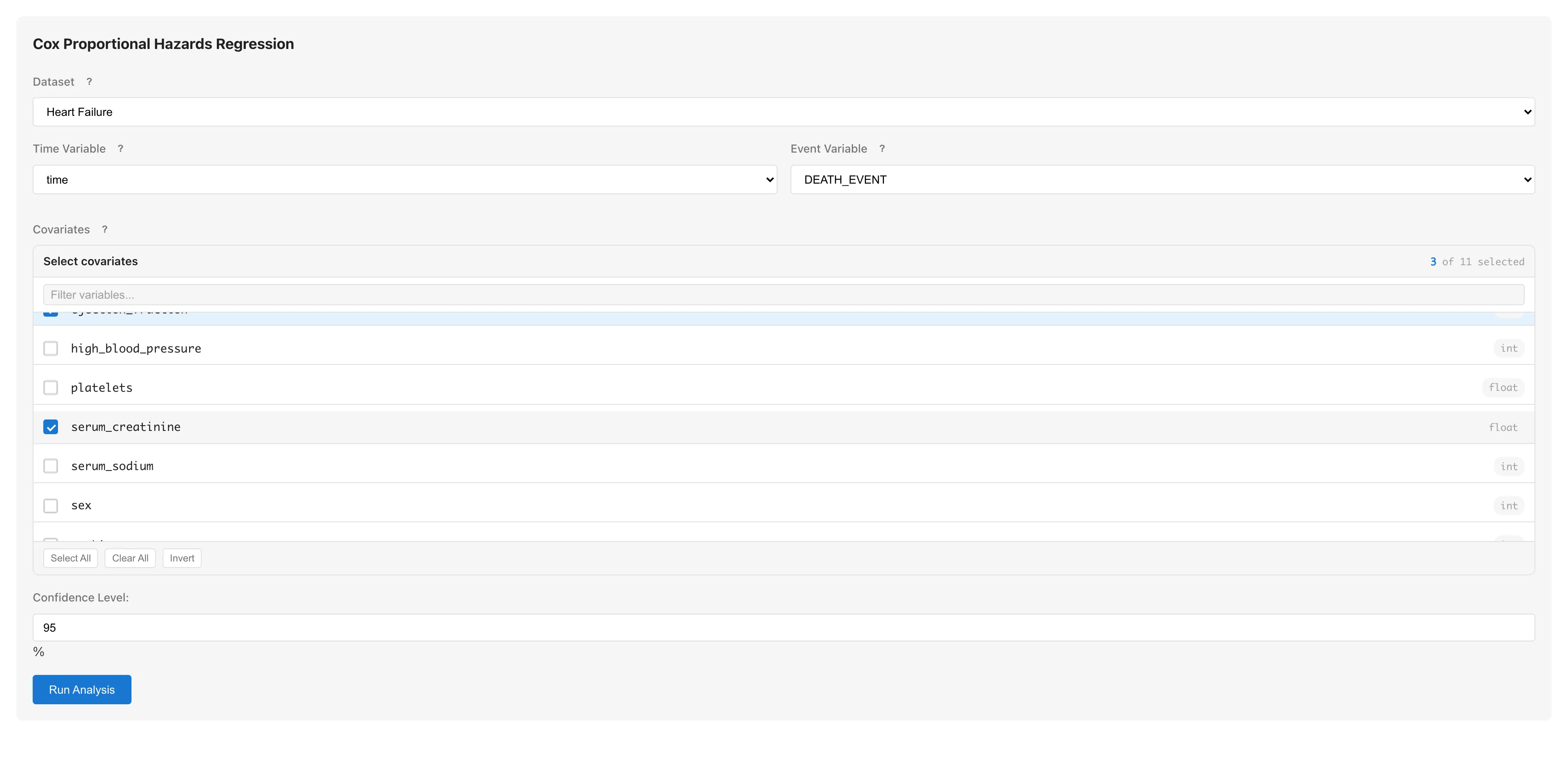
Changing the variable selection or the covariates after a run makes the displayed results no longer belong to the current settings. MIDAS removes those results from the view and shows a message asking you to run the analysis again. Restoring the previous settings brings the results back. Changing Dataset also resets the variable selection, so the results are discarded instead. Changing Confidence Level keeps the results, because that setting only recomputes the intervals from the estimated coefficients.
The displayed results also stop belonging to the current data when the dataset used for the analysis changes after a run. Reloading the dataset, editing cells, and changing an upstream dataset all count as such changes. MIDAS removes the results from the view and shows a message saying the dataset was modified. In this case there is no setting to restore, so run the analysis again to get results for the current data.
Understanding Results
Cox Proportional Hazards Regression

The upper coefficients table shows the following columns for each covariate.
| Column | Description |
|---|---|
| Variable | Variable name |
| Coef | Regression coefficient |
| SE | Standard error |
| HR | Hazard ratio |
| CI | Confidence interval for the hazard ratio. The column header reflects the selected confidence level (e.g., "95% CI") |
A hazard ratio greater than 1 indicates that an increase in the covariate raises the hazard; less than 1 indicates it lowers the hazard. See Survival Analysis Fundamentals for detailed interpretation.
Below the table, model fit metrics are reported.
| Metric | Description |
|---|---|
| Concordance Index | Harrell's C statistic. The proportion of comparable pairs where the risk score ordering agrees with the event ordering. 0.5 means no discrimination, 1.0 means perfect discrimination. The standard error in parentheses is based on the influence function |
| AIC | Akaike Information Criterion (), where is the partial log-likelihood and is the number of coefficients. Used for model comparison |
| Log Partial Likelihood | Partial log-likelihood , the basis for AIC |
| Convergence | Whether the iterative computation converged (Yes / No) and the number of iterations started |
When the iterative computation stops before meeting the convergence criterion, MIDAS does not display the values that assume the maximum partial likelihood estimate. The coefficients table has two columns, Variable and Coef at Last Iteration, and the Coef at Last Iteration column shows the coefficients at the point where the iteration stopped. These values are not estimates. The model fit metrics are limited to Log Partial Likelihood at Last Iteration, Observations / Events, and Convergence, and the adjusted survival curve, the baseline cumulative hazard, and the proportional hazards diagnostics are not displayed. The Notes section explains why the iteration stops and what to check.
Adjusted Survival Curve
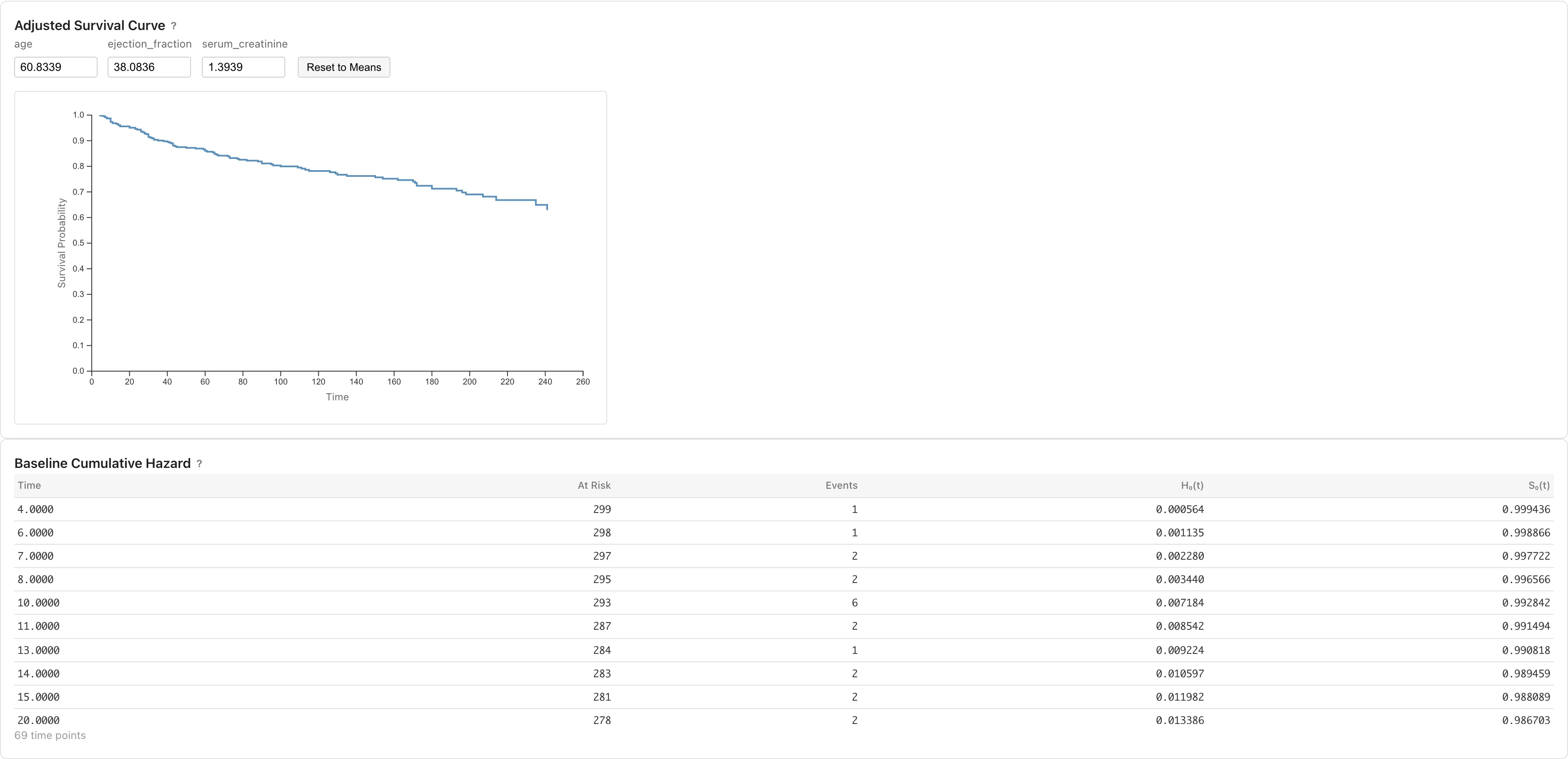
The adjusted survival curve plots predicted survival probability for a specific set of covariate values . It is computed from the baseline cumulative hazard and the estimated coefficients (formulation).
Each covariate has an input field, defaulting to the sample mean. Changing a value updates the curve immediately, so you can compare predicted survival across different covariate profiles. Reset to Means restores the defaults.
The shaded band around the curve is a pointwise confidence band for at the confidence level selected in Confidence Level, the same level as the coefficients table. A pointwise band consists of individual intervals at each time point and does not guarantee simultaneous coverage of the entire curve. The variance behind each interval combines two sources of uncertainty, the baseline hazard increments and the estimated coefficients, so the band widens toward the end of follow-up where the risk set is small, and widens further as the covariate values move away from the observed data (formulation). When the interval cannot be computed at some time points, MIDAS omits the band at those points and shows a note above the plot.
The default profile of sample means is a computational reference point, not a description of the cohort. For a binary or categorical covariate, the sample mean (for example, 0.4 for a 0/1 covariate) does not correspond to any observed individual. The curve at the mean covariate values also differs from the average of the individual survival curves. To describe a specific group, enter the covariate values that define that group.
When the survival probability cannot be computed at some time points, MIDAS omits those points from the curve and shows a note with the number of omitted points above the plot.
Baseline Cumulative Hazard
Below the adjusted survival curve, the baseline cumulative hazard table lists the following values at each event time point.
| Column | Description |
|---|---|
| Time | Event time |
| At Risk | Number of subjects in the risk set |
| Events | Number of events at this time |
| H₀(t) | Cumulative baseline hazard |
| H₀(t) nn% CI | Pointwise confidence interval for at the selected confidence level, displayed as [lower, upper] |
| S₀(t) | Baseline survival function |
| S₀(t) nn% CI | Pointwise confidence interval for , obtained from the interval for through |
The confidence intervals use the same level as the coefficients table and are the intervals of the adjusted survival curve at the all-covariates-zero profile (formulation). They are individual intervals at each time point, not a simultaneous band. A time point where the interval cannot be computed shows "-".
The baseline corresponds to all covariates set to zero. When zero is not a realistic value given the variable scales, use the adjusted survival curve with realistic covariate values (such as the sample mean) to inspect .
When the all-covariates-zero point is far from the observed data, can be 0 or 1 at every time point at the displayed precision. In this case, MIDAS displays a note above the table and points to the adjusted survival curve.
Proportional Hazards Diagnostics
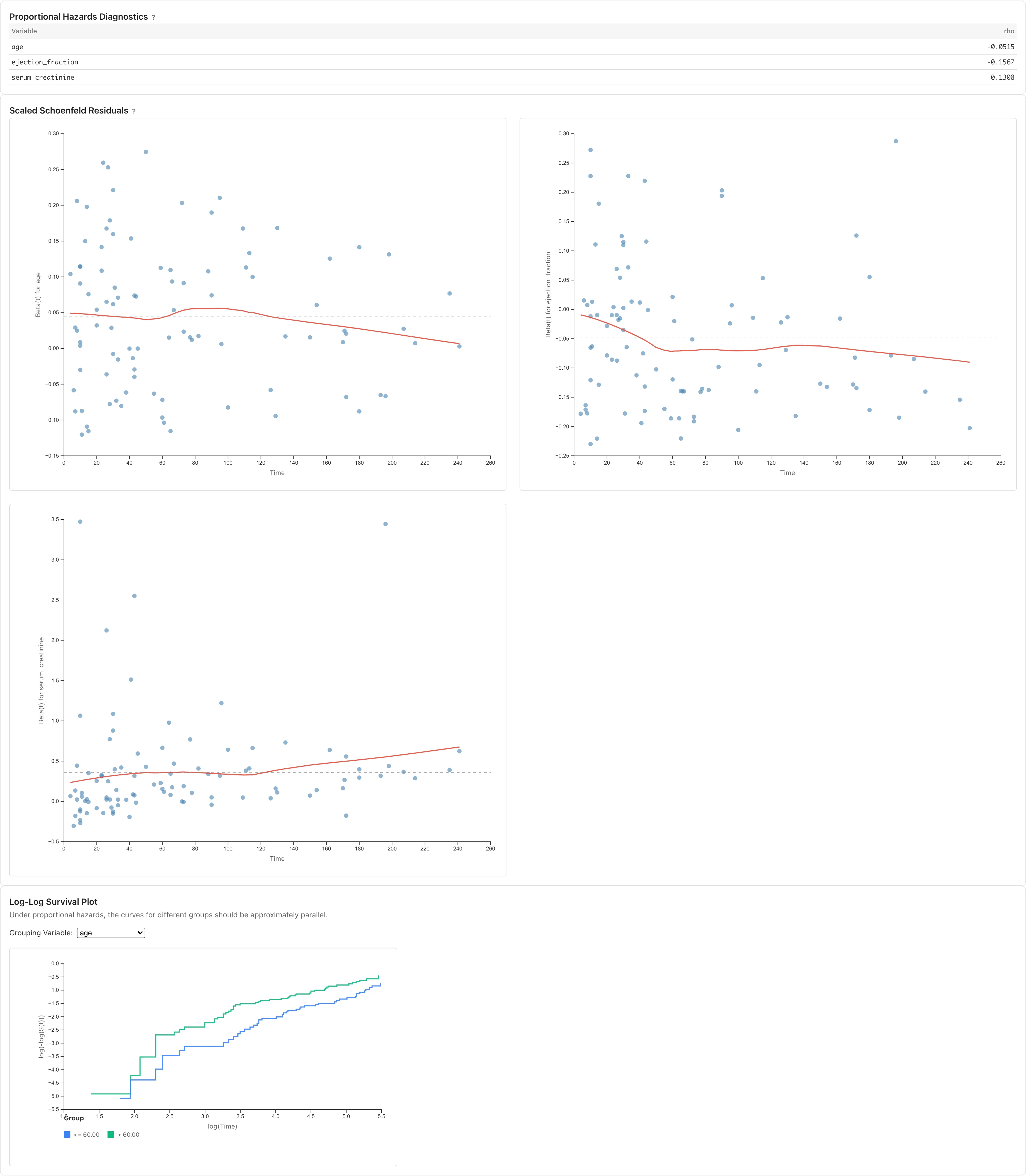
Below the coefficients table and model fit statistics, MIDAS displays diagnostics for the proportional hazards assumption. The Cox model assumes that covariate effects are constant over time — this is the proportional hazards assumption (details). When it breaks down, can only be interpreted as a weighted average over time.
Proportional Hazards Diagnostics
Displays the correlation between scaled Schoenfeld residuals and time for each covariate (Grambsch & Therneau, 1994). Uses the KM time transformation .
| Column | Description |
|---|---|
| Variable | Variable name |
| rho | Pearson correlation between scaled Schoenfeld residuals and a Kaplan-Meier-based time transform. Values close to 0 are consistent with the assumption |
Covariates with a large absolute rho may have effects that change over time. Since rho alone does not reveal the pattern or severity of the departure, inspect the Schoenfeld residual plots below. MIDAS uses rho together with visual inspection of the plots, and does not display a test statistic or p-value.
MIDAS cannot always compute rho. The denominator of the Pearson correlation is zero when either the scaled Schoenfeld residuals or the time transform is constant. This happens when fewer than two events are observed, and when all events occur at the same time. MIDAS shows rho as "-" in these cases.
Scaled Schoenfeld Residuals
For each covariate, plots scaled Schoenfeld residuals against time. The red curve is a LOESS smooth; the dashed gray line is the estimated coefficient . Under proportional hazards, residuals scatter randomly around and the LOESS line stays close to horizontal. An upward or downward trend in the LOESS line indicates that the covariate's effect varies over time.
Log-Log Survival Plot
Plots group-specific Kaplan-Meier estimates as versus . Select the grouping covariate from the Grouping Variable dropdown. When the selected covariate has five or fewer distinct values, each value forms its own group; with six or more, observations are split into two groups at the median, and values equal to the median go to the "<=" group. When the median equals the maximum, no observation falls in the ">" group and only one group forms. In that case, and when a group has fewer than two event times at which the survival probability is strictly between 0 and 1, MIDAS shows a notice above the plot. In the first case there are no curves to compare; in the second, the group has no curve and no legend entry.
When the hazards of two groups are proportional, their curves are parallel, separated vertically by the log hazard ratio. The Kaplan-Meier estimates vary around these curves, and the variation grows at times when few subjects remain at risk. Crossings or changes in separation near the ends of the curves can therefore come from sampling variation.
This parallelism is not the same as the model's proportional hazards assumption. The model's assumption is conditional on all covariates, whereas each curve is estimated within its group and is not adjusted for the other covariates in the model. When other covariates affect the hazard, or a group combines different covariate values as in a median split, the group curves need not be parallel even if the assumption holds. Conversely, parallel curves do not show that the assumption holds.
The median split is a convenience that discards some information from the continuous variable and may miss (or exaggerate) non-proportionality at the continuous scale. For continuous covariates, the Schoenfeld residual plot above is better suited for diagnosing the proportional hazards assumption.
When the diagnostics above suggest a violation of the proportional hazards assumption, approaches such as stratified Cox models or time-dependent covariate models can address it, but MIDAS does not currently support them. Interpret results with care, considering the severity of the violation and the goals of the analysis. If the goal is to compare groups defined by a single categorical variable, Kaplan-Meier with RMST is an alternative that does not rely on the proportional hazards assumption, although it cannot adjust for covariates.
Notes
- Tied events (multiple events at the same time) are handled using the Efron method (details)
- When the fit does not converge: The iterative computation that maximizes the partial likelihood can stop before meeting the convergence criterion for one of three reasons, and MIDAS shows the applicable reason in a warning. The first is that the number of iterations reached the limit of 100. The second is that each of the 10 step lengths tried along the update direction decreased the partial log-likelihood by more than the acceptance threshold. The acceptance threshold is times one plus the absolute value of the partial log-likelihood at the previous iteration. The third is that the information matrix could not be solved, so the update direction could not be computed. When a coefficient at the point where the iteration stopped changes the log hazard ratio by more than 10 across the observed range of its covariate, the warning names that covariate. Check for nearly collinear covariates, for a covariate that nearly determines which subject has the event at each event time, and for too few events relative to the number of covariates. When separation, a singular information matrix, or a variance that is not a finite positive value is found at the point where the iteration stopped, MIDAS displays that error instead of a result that did not converge
- Separation (monotone likelihood): When a covariate separates the event ordering so strongly that its coefficient diverges, the partial likelihood has no finite maximum and the estimate does not exist. MIDAS stops the fit and reports an error that names the affected covariates. Check whether a covariate, or a category of one, perfectly determines which subject has the event at each event time, and whether there are too few events for the number of covariates. Remove or combine the separating covariate, or reduce the number of covariates, then refit
- Signs of separation (warnings): Even when the fit succeeds and returns coefficients with standard errors, estimates on data close to separation may not be reliable. MIDAS displays the results with a warning when a coefficient estimate is extreme and its standard error is large enough to cover the estimate, when the same condition holds only along a combination of covariates, or when the partial likelihood converged before the coefficients stabilized. For the terms or combination of covariates the warning points to, the standard errors and confidence intervals cannot be trusted. When the fit converged before the coefficients stabilized, the coefficients and hazard ratios themselves may also be unreliable. The detection is tuned conservatively to avoid false warnings on legitimate strong effects, so the absence of a warning does not mean there are no signs of separation. Check the data from the same viewpoints as for the separation error
- Non-finite variance: When a covariate spans an extreme range, the variance computation can overflow or become undefined, so the standard errors cannot be computed and the fit stops with an error. Rescale or standardize the covariates, then refit
- Rows with missing values in the time, event, or any covariate variable are automatically excluded (listwise deletion; see Missing Data Mechanisms for validity conditions). When rows are excluded, the results show how many. Rows dropped for a missing time or event value are reported separately from rows dropped for a missing covariate.
See also
- Survival Analysis Fundamentals - Mathematical background of time-to-event data, Kaplan-Meier, and Cox model
- The Kaplan-Meier Tab - Estimating survival curves and comparing groups with RMST
- Tutorial: Kaplan-Meier Analysis - A practical example with sample data
References
- Grambsch, P. M. and Therneau, T. M. (1994). Proportional hazards tests and diagnostics based on weighted residuals. Biometrika, 81(3), 515--526. https://www.jstor.org/stable/2337123
Also available as a Markdown file.