Prediction Accuracy Metrics

Prediction accuracy metrics summarize how good a model's predictions are by comparing predicted values with observed values.

The appropriate metric depends on the type of response. Metrics that measure the size of errors suit continuous responses, while binary responses call for dedicated metrics that evaluate predicted values between 0 and 1.

The values of these metrics also depend on which data are used for evaluation. The model chooses its coefficients to fit the fitting data as closely as possible. Metrics evaluated on the same data therefore come out better than values evaluated on new data. Fitting the chance variation in the data as well is called overfitting, and the stronger the overfitting, the larger this gap. To learn how well the model predicts new data, evaluate on data not used for fitting.

RMSE and MAE

RMSE (Root Mean Squared Error) and MAE (Mean Absolute Error) summarize the size of prediction errors. Both values are expressed in the same unit as the response variable.

\text{RMSE} = \sqrt{\frac{1}{n}\sum_{i=1}^{n}(y_i - \hat\mu_i)^2} \qquad \text{MAE} = \frac{1}{n}\sum_{i=1}^{n}\lvert y_i - \hat\mu_i \rvert

The denominator of the RMSE is the number of observations $n$ . The residual standard error shown on the Linear Regression tab divides the same sum of squared errors by the residual degrees of freedom $n-p$ , which makes it a different quantity whose value differs for the same model unless that sum is 0.

The two metrics differ in their sensitivity to large errors. RMSE squares the errors before averaging, so large errors count more heavily. MAE averages the absolute errors as they are. On the same data, RMSE is always at least as large as MAE, and a few large errors increase RMSE more. A large gap between the two indicates that the size of the errors varies widely across observations.

R² and Predictive R²

R² is the fraction by which the squared error is reduced compared with a baseline model that predicts the mean of the observed values.

R^2 = 1 - \frac{\sum_i (y_i - \hat\mu_i)^2}{\sum_i (y_i - \bar{y})^2}

Values near 1 indicate small errors. A value of 0 indicates predictions no better than the mean, and negative values indicate predictions worse than the mean¹.

The R² that MIDAS shows in the GLM Prediction tab and in the GLM tab's fitting results is in both cases a predictive R², using the mean $\bar{y}$ of the observed values in the data being evaluated as the baseline. The fitting-results metrics evaluate the fitting data itself, so they are in-sample values that directly reflect the fit, unlike a prediction against a different dataset. Even when the R² on the fitting data is positive, the predictive R² on new data can be negative.

Responses with Mean-Dependent Variance and Mean Deviance

For families whose variance depends on the mean (Poisson with $V(\mu) = \mu$ , Gamma with $V(\mu) = \mu^2$ , and so on), metrics based on squared error are misleading as a measure of fit. For this reason, MIDAS does not show R² for these families. Metrics based on squared error average the errors of all observations with equal weight. In these families, observations with larger means naturally vary more. Observations with large means therefore account for most of the sum of squared errors, and R² mostly reflects the fit to those observations.

Mean Deviance is the deviance $D$ on the evaluation data divided by the number of observations $n$ .

\text{Mean Deviance} = \frac{D}{n}

Because the deviance measures the discrepancy between observations and predictions through the family's likelihood, it summarizes the errors without being skewed toward large-mean observations even for families whose variance depends on the mean. Smaller values indicate predictions closer to the observations². The scale of the value depends on the unit of the response and on the family, so there is no standalone threshold for a good value. Use it to compare models on the same family and the same evaluation data.

Brier Score

A model for a binary response outputs a predicted value between 0 and 1 for each observation. The Brier Score evaluates this predicted value as the probability of a 1. It is computed as the mean squared difference between the observed values (0 or 1) and the predicted values.

\text{Brier} = \frac{1}{n}\sum_{i=1}^{n}(y_i - \hat{p}_i)^2

Values near 0 indicate predicted values close to the observations. The reference level is a prediction that does not distinguish observations and assigns the proportion of 1s, $\bar{y}$ , to every observation. Its Brier Score is $\bar{y}(1-\bar{y})$ . This is at most 0.25, reached when 1s and 0s are equally frequent, and shrinks as the proportion becomes unbalanced. A model whose Brier Score is at or above this level does not improve on predicting the proportion uniformly.

The ROC Curve and AUC

Turning predicted values into 0/1 decisions creates two kinds of errors that trade off against each other depending on the threshold. A decision is made by choosing a threshold. Observations whose predicted value exceeds it are classified as 1, and the rest as 0. The two kinds of errors are classifying a 0 observation as 1, and missing a 1 observation by classifying it as 0. Lowering the threshold classifies more observations as 1, so fewer 1s are missed. In exchange, more 0s are classified as 1.

The ROC curve draws this whole trade-off as a single curve. It plots the fraction of 0 observations classified as 1 on the horizontal axis and the fraction of 1 observations classified as 1 on the vertical axis. The points traced as the threshold moves from the maximum to the minimum form the curve. The curve runs from the bottom-left point, where no observation is classified as 1, to the top-right point, where every observation is. The better the model discriminates, the more 1s it detects before misclassifying many 0s, so the curve approaches the top-left corner.

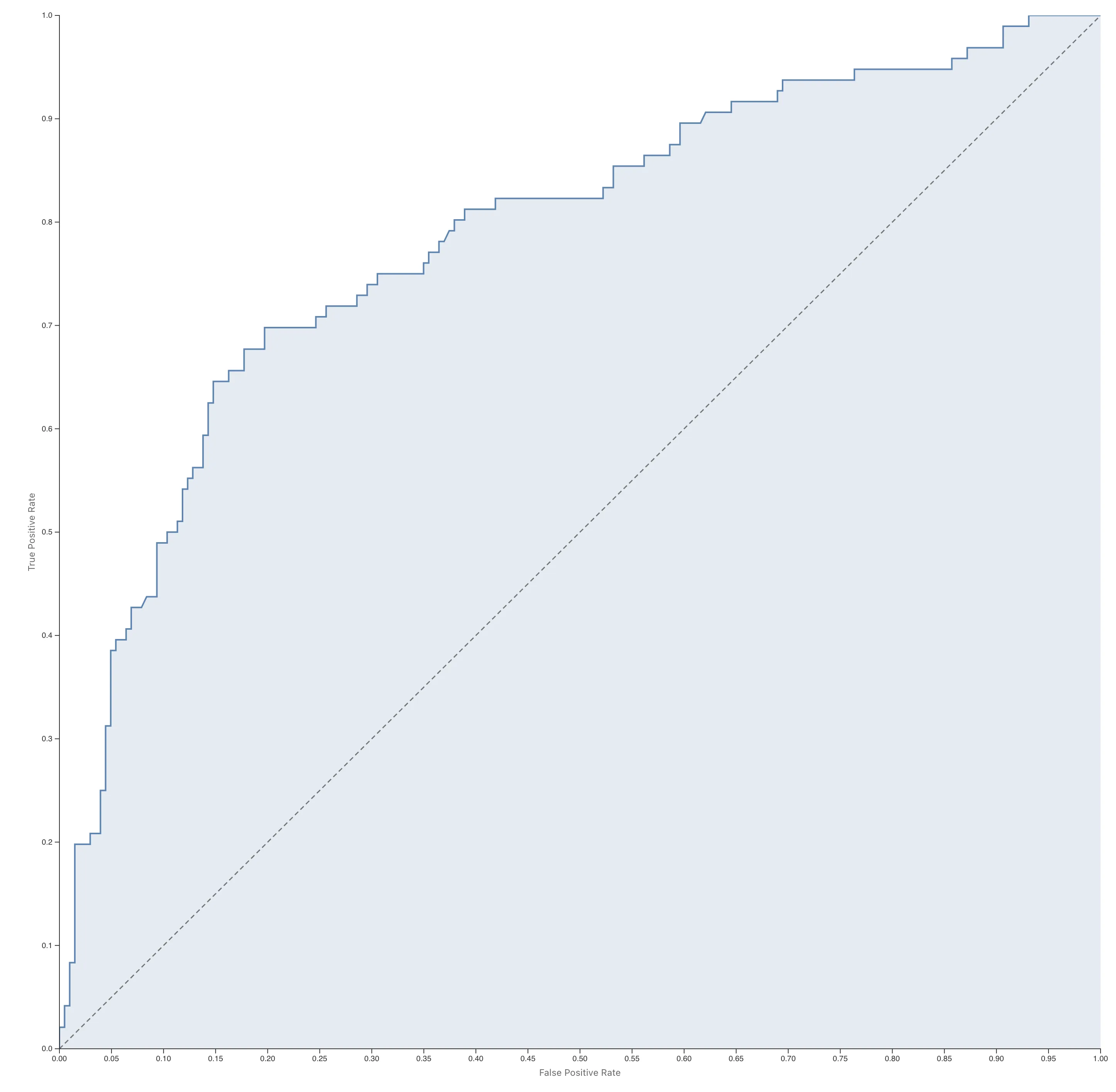
ROC curve of a Binomial GLM fitted to the Heart Failure data

The figure shows the ROC curve of a Binomial GLM that predicts death (the DEATH_EVENT column) in the Heart Failure sample data from age, ejection_fraction, and serum_creatinine. The predicted values are predictions for the same data the model was fitted to. The dashed diagonal corresponds to random assignment: when observations are classified as 1 with a fixed probability regardless of the predicted values, both the fraction of 0 observations classified as 1 and the fraction of 1 observations classified as 1 equal that probability.

AUC (Area Under the Curve) is the area under the ROC curve and summarizes the model's ability to discriminate without depending on the choice of threshold. In the figure above, the shaded region is this area. A value of 1.0 means some threshold classifies every observation at or below it as 0 and every observation above it as 1, discriminating perfectly. A value of 0.5 means the assignment is no better than random. Which threshold to choose is a decision outside the analysis, made by weighing the two kinds of errors against each other. AUC measures how good a trade-off the model can achieve before that decision is made.

AUC uses the predicted values only as scores to compare against the threshold and does not evaluate them as probabilities. For example, a model that assigns 0.9 to every observation with outcome 1 and 0.8 to every observation with outcome 0 discriminates perfectly with a threshold of 0.85, so its AUC is 1.0. The Brier Score of the same model, however, is 0.325 on data with half 1s and half 0s, worse than the 0.25 of a prediction that assigns 0.5 to every observation. To assess the accuracy of the probability values, use the Brier Score.

For models fitted in the successes-and-trials form (Grouped Binomial), each row is treated as its number of trials of 0/1 observations, and the Brier Score and AUC are weighted by the number of trials. Per-observation 0/1 data corresponds to the case of one trial and is computed with the same formulas.