The ARIMA Tab
The ARIMA tab fits an ARIMA model to a single numeric column treated as a time series. An ARIMA(p,d,q) model differences the series d times and then expresses each value as a linear combination of the p preceding values (the autoregressive part, AR) and the q preceding error terms (the moving-average part, MA). The orders p, d, q can be specified manually or selected automatically. Specifying a seasonal period turns the model into ARIMA(p,d,q)(P,D,Q)[s] with seasonal orders. This model is called seasonal ARIMA, or SARIMA. The automatic order selection procedure and its theoretical background are explained in Automatic ARIMA Order Selection.
The ARIMA tab reads the series in the row order of the dataset. There is no time column to specify, and the observations are assumed to be equally spaced. If the rows are not in time order, prepare a sorted dataset first, for example with the SQL Query Editor tab.
Basic Usage
The examples below use the Bike Sharing (Daily) dataset. Opening the link launches MIDAS with this dataset loaded.
Opening ARIMA
Select Analysis > ARIMA... from the menu bar.
Setting Up the Model
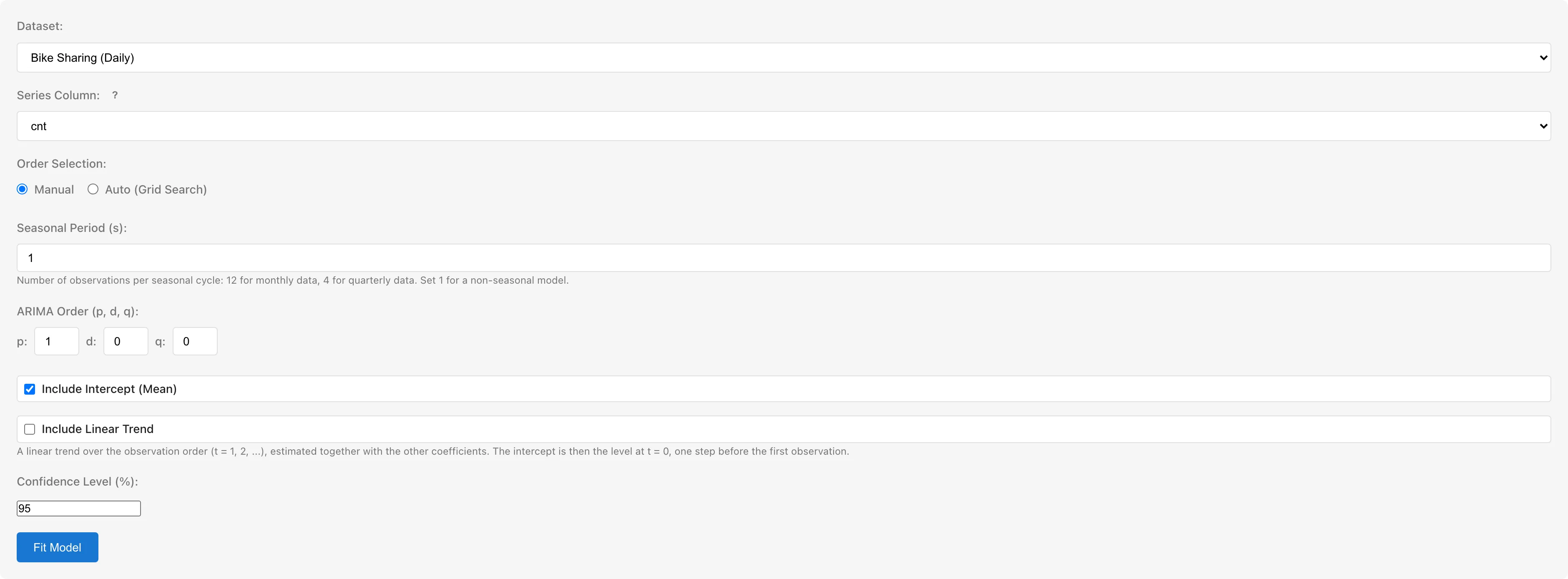
Dataset selects the dataset to analyze.
Series Column selects the column to use as the series. Only numeric (interval or ratio scale) columns can be selected.
Order Selection chooses how the orders are set. Manual specifies the orders directly; Auto (Grid Search) selects them automatically. The default is Manual.
Seasonal Period (s) is the number of observations per seasonal cycle: 12 for the yearly cycle of monthly data, 4 for quarterly data. Setting it to 1 gives a model with no seasonal component. The default is 1.1
Specifying the Order Manually
ARIMA Order (p, d, q) sets the three orders: p is the number of autoregressive terms, from 0 to 5; d is the differencing order, from 0 to 2; q is the number of moving-average terms, from 0 to 5. The default is (1, 0, 0).
When Seasonal Period is 2 or more, Seasonal Order (P, D, Q) is also specified: P is the number of seasonal autoregressive terms, from 0 to 2; D is the seasonal differencing order, 0 or 1; Q is the number of seasonal moving-average terms, from 0 to 2. The default is (0, 0, 0).
Automatic Order Selection
Auto (Grid Search) sets the differencing orders first with stationarity tests, then selects the remaining orders by fitting every combination of candidates under that differencing. The differencing order d is set with the KPSS test. In seasonal models, the seasonal differencing order D is set before that with the OCSB test. Among the fitted candidates, p and q — and P and Q in seasonal models — are chosen to minimize the selection criterion. For why the differencing orders alone are set by tests rather than by AIC or BIC, see Automatic ARIMA Order Selection.
Search Range sets the search limits for p, d, q. The defaults are max p = 3, max d = 1, max q = 3.
When Seasonal Period is 2 or more, Seasonal Search Range sets the search limits for the seasonal orders P and Q. Both default to 1. The seasonal differencing order D is chosen automatically by an OCSB test, so it has no input field.
Selection Criterion chooses between AIC and BIC. The default is AIC.
Constant and Trend Terms
The meaning and label of the constant-term checkbox change with the total differencing d + D. At d + D = 0 the label is Include Intercept (Mean) and the constant is the mean of the series. At d + D = 1 the label is Include Drift and the constant is the mean of the differenced series, the drift. With an ordinary difference (d = 1) it is the average change per period of the original series, and with a seasonal difference alone (D = 1) it is the average change per s periods. At d + D of 2 or more the checkbox is disabled and no constant is estimated, because the constant would then correspond to a polynomial trend of degree d + D in the original series. In Auto, the differencing orders are decided at run time, so the label is Include Intercept or Drift. The default is on.
Include Linear Trend adds a linear trend term over the observation order t = 1, 2, ... to the model. Its slope is estimated as a separate parameter only at d + D = 0. At d + D = 1 the trend is absorbed into the drift term: the drift equals the slope with an ordinary difference, and the slope multiplied by s with a seasonal difference alone. At d + D of 2 or more the trend is removed by differencing. Specifying these orders in Manual therefore disables the checkbox.2 Turning it on in Auto switches the KPSS test on the undifferenced series to the variant whose null hypothesis is trend stationarity. For what this switch means, see Automatic ARIMA Order Selection: Why the sequential procedure works. The default is off.
Confidence Level (%) sets the level of the coefficient confidence intervals. The default is 95, and the range is 50 to 99.99. The chosen level appears in the Lower N% / Upper N% columns of the coefficient table.
Running the Analysis
Clicking Fit Model starts the estimation. The coefficients are estimated by maximum likelihood. While running, the button reads Fitting..., and in Auto the number of fitted candidates is shown as (current/total). Cancel stops the estimation.
Changing the series column, the orders, the seasonal period, or the constant and trend settings after a run makes the displayed results no longer belong to the current settings. MIDAS removes those results from the view and shows a message asking you to run the analysis again. Restoring the previous settings brings the results back. Changing Dataset also resets the column selection, so the results are discarded instead. Changing Confidence Level keeps the results, because that setting only recomputes the intervals from the estimated coefficients.
The displayed results also stop belonging to the current data when the dataset used for the estimation changes after a run. Reloading the dataset, editing cells, and changing an upstream dataset all count as such changes. MIDAS removes the results from the view and shows a message saying the dataset was modified. In this case there is no setting to restore, so run the analysis again to get results for the current data.
Understanding Results
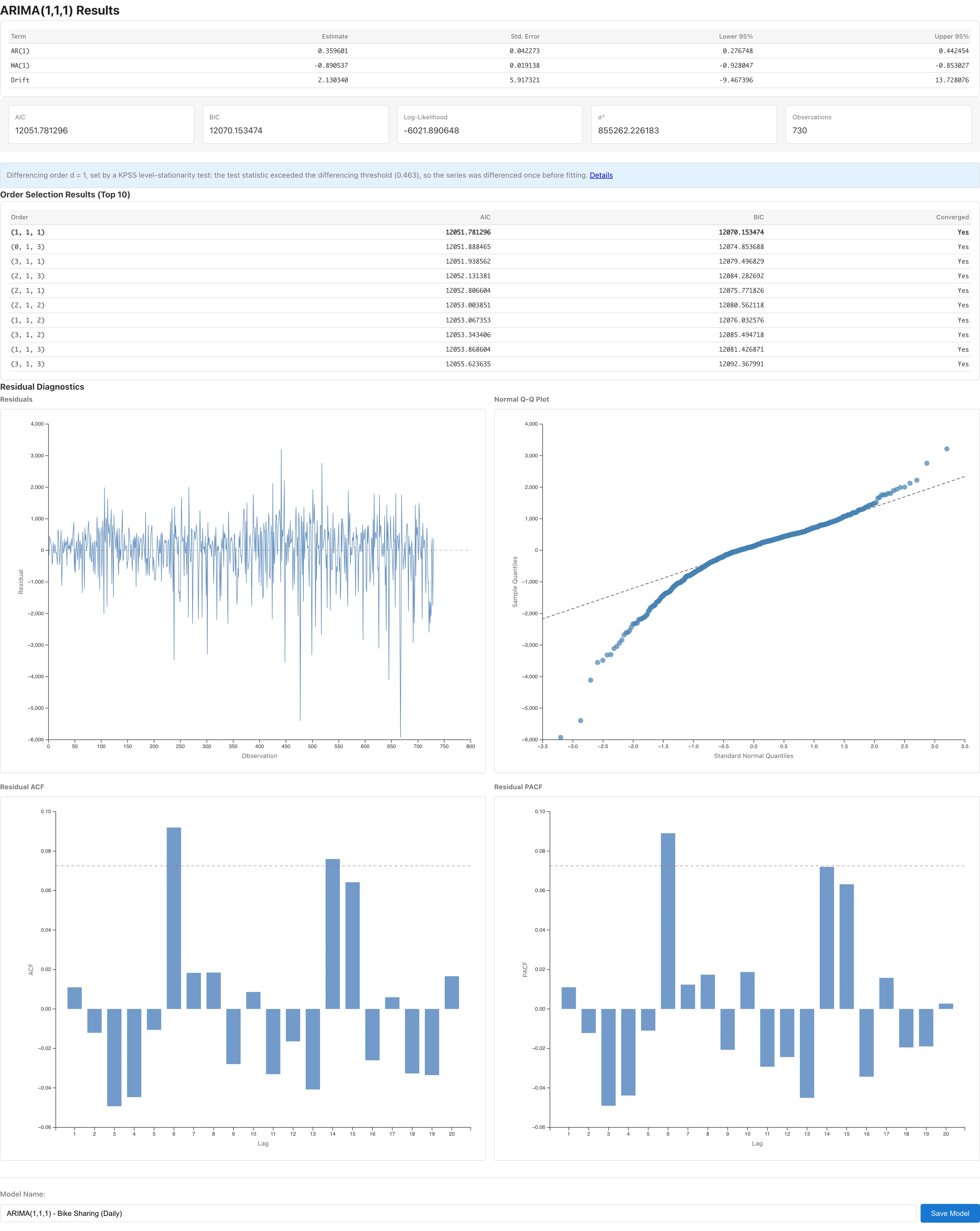
The results heading shows the fitted order, as in "ARIMA(1,0,0) Results". For seasonal models it includes the seasonal order and period, as in "ARIMA(1,0,0)(1,1,0)[12] Results".
Coefficients
The coefficient table shows the following columns.
| Column | Contents |
|---|---|
| Term | The coefficient term. AR(1), AR(2), ... are autoregressive coefficients; MA(1), ... are moving-average coefficients; SAR(1), ... and SMA(1), ... are seasonal autoregressive and seasonal moving-average coefficients. The constant appears as Intercept at d + D = 0 and as Drift at d + D = 1. The slope of the linear trend appears as Trend. |
| Estimate | The coefficient estimate |
| Std. Error | The standard error |
| Lower N% / Upper N% | Normal-approximation confidence interval. N is the chosen confidence level. |
A coefficient whose standard error could not be computed shows "-" in the Std. Error and confidence interval columns. A warning to that effect appears above the results.
Fit Statistics
Below the coefficient table, AIC, BIC, Log-Likelihood, σ², and Observations are shown. σ² is the estimate of the error-term variance. Observations is the number of observations in the differenced series used in the fit. It is d + sD fewer than the number of values in the series after the exclusion described in Automatic Exclusion of Missing and Invalid Values. When the estimation did not converge, the likelihood is not maximized and a value computed from it would not be the AIC or BIC of the model, so AIC and BIC show "-".
Comparing AIC and BIC is meaningful only between models with the same differencing orders d and D. With different differencing, the data the likelihood is computed on changes, so the ordering of AIC or BIC values says nothing about which model is better. For the reason, see Automatic ARIMA Order Selection: Why d alone is selected by a test.
Notes on the Selected Orders
In Auto, a note next to the results explains how the differencing orders were set. It states the selected orders and whether the KPSS statistic — and the OCSB statistic in seasonal models — exceeded the differencing threshold. MIDAS reports only this fact; it displays no p-values and no significant/not-significant verdicts.
When a statistic cannot be computed — for example, the series is constant, or too short for the seasonal period — the note states this instead, and the series is modeled without that differencing.
If a constant or trend term was requested but not estimated, a note explaining the reason is also shown.
Lists of Searched Candidates
When Auto fits more than one candidate, the candidates compared by the selection criterion and the candidates excluded from the comparison are shown in separate lists. Order Selection Results (Top 10) sorts the candidates whose estimation converged in ascending order of the selection criterion and shows the top 10. The columns are Order, AIC, BIC, and Status, and the row of the selected model is bold. Every candidate in this list has the Status Converged.
Candidates Excluded from Selection shows every candidate excluded from the selection, however many there are. The columns are Order and Status, and the Status is either Not converged or Failed. Candidates whose estimation did not converge (Not converged) are excluded from the selection because their likelihood is not maximized, so a value computed from it would not be the AIC or BIC of the model. The candidates in this list have no AIC or BIC, so the list has no AIC or BIC columns. When no candidate is excluded, this list is not shown.
Candidates that could not be fitted at all (Failed) are excluded from the selection for a different reason than non-convergence. A non-converged candidate is one whose iteration stopped without meeting the convergence criterion, and a different order or differencing order may converge. A Failed candidate is one for which the model of that order could not be built from this data, for example because too few observations remain after differencing, the differenced series has zero variance, or the likelihood cannot be evaluated. The Status column shows the reason.
When one or more candidates did not converge or failed, a note above the lists states the total number of candidates and, separately, how many did not converge and how many could not be fitted. If no searched candidate converged or could be fitted, no candidate was compared, so Order Selection Results (Top 10) is not shown. In that case the note states that the model shown is not a result of the selection criterion comparison but the ARIMA(0,d,0) fallback MIDAS fits when no candidate can be compared.
Residual Diagnostics
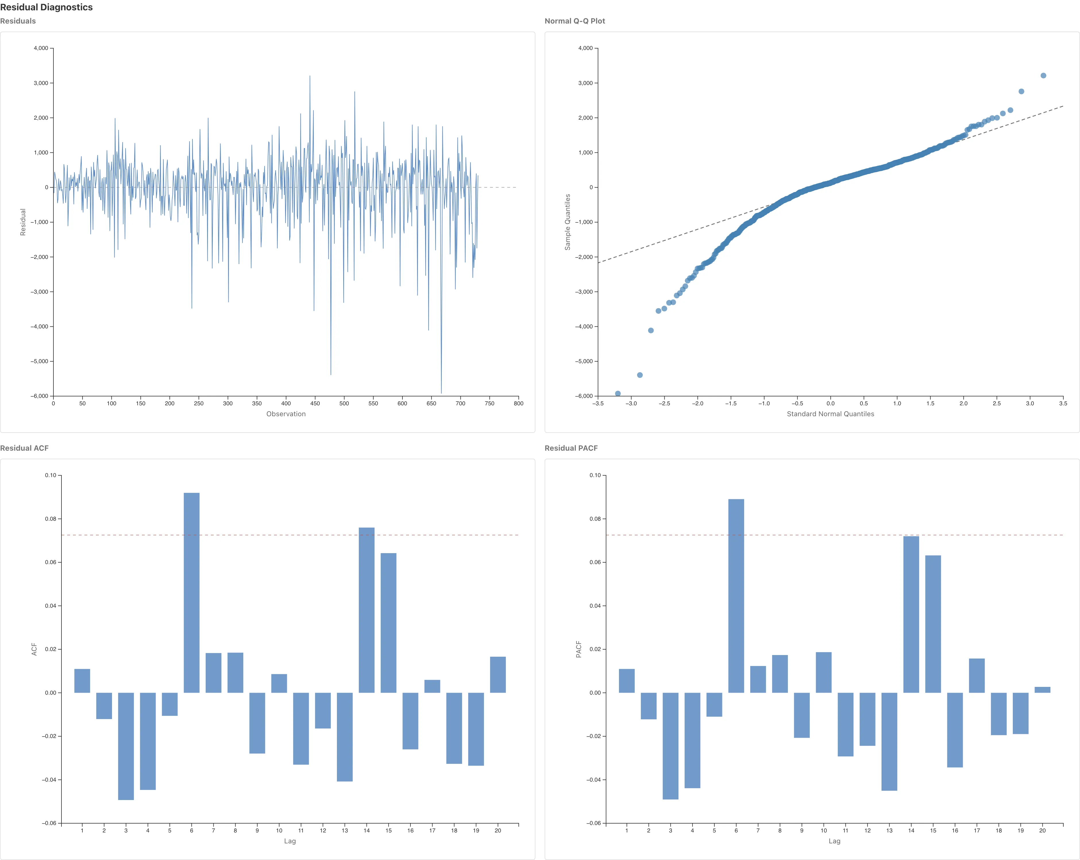
The four plots under Residual Diagnostics at the bottom of the results show whether the model has explained the autocorrelation of the series. The residuals are the variation the model did not explain: if the model captures the autocorrelation of the series, they approach an uncorrelated series.
Residuals plots the residuals in observation order. The dashed line marks zero. If the model is adequate, the residuals scatter around zero with a constant spread. A spread that changes over time suggests the constant-variance assumption does not match the data.
Normal Q-Q Plot plots the residual quantiles against theoretical normal quantiles. Points along the straight line indicate that the residual distribution is close to normal. The coefficient confidence intervals rest on a normal approximation, so treat them with caution when the departure from the line is large.
Residual ACF and Residual PACF show the autocorrelation and partial autocorrelation functions of the residuals up to lag 20. The dashed band is ±1.96/√n, where n is the number of observations — a guide to the range within which the sample autocorrelations of an uncorrelated series fall with asymptotic probability of about 95%. If the autocorrelations at many lags fall outside the band, the model has not fully explained the autocorrelation of the series, and increasing the orders or revisiting the seasonal period is worth considering. The band is a guide: even for an uncorrelated series, about one lag in 20 falls outside it. The band is also based on the variance 1/n that applies when the observed series itself is uncorrelated. For the residuals of a fitted model, the variance of the sample autocorrelation at low lags is smaller than 1/n, so at low lags the band is wider than the actual variability and can miss autocorrelation remaining in the residuals. When the residuals have zero variance and the sample autocorrelation is undefined, a note saying so replaces the plot.
Saving the Model
Enter a model name in Model Name and click Save Model. The name is generated automatically in the form "ARIMA(1,0,0) - dataset name" and can be used as is.
Saving the model reveals two buttons: View Model Details and Save Coefficients as Dataset.
View Model Details opens the Model Detail tab, which shows the saved model's coefficient table, fit statistics, and residual ACF and PACF without refitting.
Save Coefficients as Dataset saves the coefficient table as a dataset. The saved dataset has the columns Term, Estimate, Std. Error, Lower N%, and Upper N%, and can be exported to CSV.
Notes
Automatic Exclusion of Missing and Invalid Values
Missing values (null), non-numeric values, and infinities are excluded from the series automatically. In a time series, this exclusion differs in kind from the listwise deletion of the other tabs: the remaining observations are treated as a contiguous series, so a gap in the middle of the series makes observations that are actually far apart in time adjacent. See Missing Data Mechanisms for details.
When values are excluded, a warning above the results shows how many were removed and whether the time spacing is kept. If all of them were at the start or end of the series, the warning states that the remaining values keep their original time spacing. If some of them were inside the series, the warning gives their number and states that lags spanning a removed value do not match the original time spacing. When the model has seasonal terms and the values after a removed value move to a different position in the seasonal cycle, the warning states that as well. The position does not move when the number of values removed up to that point is a multiple of the seasonal period s. The same warning appears in the Model Detail tab of the saved model.
If fewer than 10 valid observations remain after the exclusion, an error such as "Only 8 valid numeric observation(s) remain after removing 3 missing or non-finite value(s). ARIMA requires at least 10." is shown and no estimation runs.
Estimation Warnings
If the estimation does not converge, the warning "Model did not converge. Results may be unreliable." is shown3. The coefficients and standard errors are then not reliable. Consider reducing the orders, changing the differencing order, or switching to Auto.
If a root of the estimated autoregressive component is close to the unit circle, a warning states that the autoregressive component is near-nonstationary and that estimates and their normal-approximation confidence intervals near this boundary may be unreliable. The warning does not go on to suggest a change to the model. An AR coefficient estimated very close to 1 is the typical sign of too little differencing, so consider increasing the differencing order d.
If a root of the estimated moving-average component is close to the unit circle, a similar warning is shown. When this appears to result from too much differencing, the warning includes a suggestion to reduce the differencing order by 1. For how too little and too much differencing each destabilize the estimation, see Automatic ARIMA Order Selection: Why the sequential procedure works.
If a distinctly different set of coefficients fits the data almost as well as the reported one, a warning states that the coefficients are weakly identified. MIDAS maximizes the likelihood from several starting points and reports the best fit found; the warning appears when another optimization run reaches a nearly equal log-likelihood with clearly different coefficients. The absence of this warning does not guarantee that the coefficients are well identified, because the detection is limited to the alternative solutions that the finite set of starting points reaches. The reported coefficients and their confidence intervals do not convey this ambiguity. This state typically arises when autoregressive and moving-average factors nearly cancel, in the seasonal or the non-seasonal terms; the warning suggests reducing the orders on the side where the coefficients differ.
Related Pages
- Automatic ARIMA Order Selection -- why the differencing orders are set by tests, and the background of the KPSS and OCSB tests
- Agent API (window.midas) -- how to run ARIMA from
models.run() - Missing Data Mechanisms -- how the exclusion of missing values affects the estimation
Footnotes
-
Estimation slows down as the seasonal period grows. With a period of 52 or more, a single fit can take seconds to minutes, and an Auto grid search repeats this fit for every candidate. The form shows a notice to that effect, and a running fit can be cancelled with Cancel. ↩
-
With the trend term on, the Intercept represents the level at t = 0 — one step before the first observation — rather than the mean of the series. The constant-term label also changes from Include Intercept (Mean) to Include Intercept. Turning the constant term off and the trend term on constrains the mean function to 0 at t = 0. The slope then carries the level of the series as well as its change per period, so for a series whose level is far from 0 the slope estimate cannot be read as a rate of change. ↩
-
Convergence means that the iteration stopped after meeting the convergence criterion: either the gradient of the log-likelihood is small enough, or the log-likelihood cannot be increased further along the direction searched. When the point reached lies on the boundary of the stationarity and invertibility region (a partial autocorrelation with absolute value 0.999 or more), MIDAS also evaluates the log-likelihood at the points where each boundary partial autocorrelation is moved inward by 0.001, one at a time, and does not treat the criterion as met if the log-likelihood is larger there. The point reached is a local solution, and it is not guaranteed to be the global maximum of the log-likelihood. ↩
Also available as a Markdown file.