Linear Regression

The Linear Regression tab performs ordinary least squares (OLS) linear regression analysis. OLS finds the coefficient vector $\hat\beta = (X'X)^{-1}X'Y$ that minimizes the residual sum of squares. See Regression Analysis Fundamentals for the mathematical background.

For count data, binary outcomes, or other non-normal response variables, use Generalized Linear Model (GLM) instead.

Basic Usage

Opening Linear Regression

Select Analysis > Linear Regression (OLS)... from the menu bar to open a new Linear Regression tab.

Setting Up Variables

Variable setup

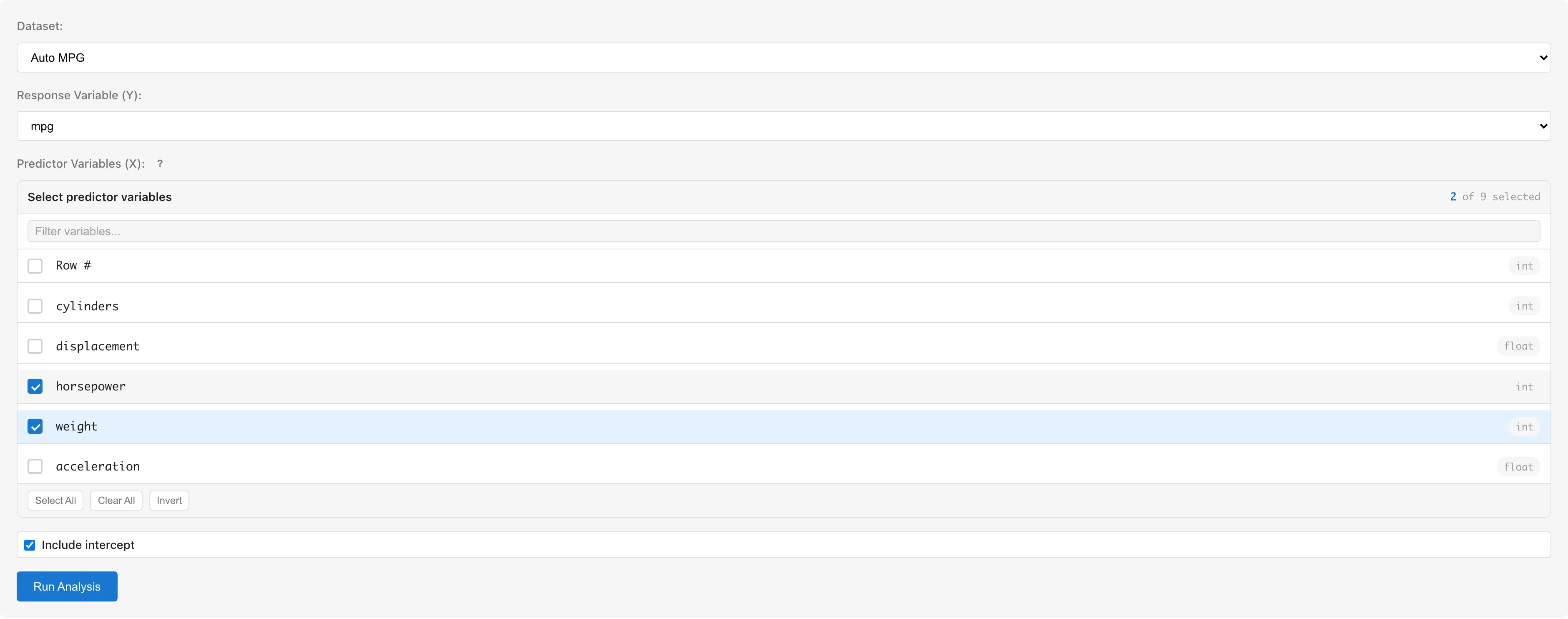
Dataset selects the dataset to analyze.

Response Variable (Y) selects the response variable. Only numeric columns (int64, float64) are available.

Predictor Variables (X) selects predictor variables using checkboxes. Only numeric columns are selectable; non-numeric columns are grayed out. To use categorical variables, convert them to numeric dummy variables using the Dummy Coding tab first (see Notes).

Include intercept toggles the intercept term. Enabled by default.

Click the Run Analysis button to run the analysis.

Understanding Results

Model Summary

Analysis results

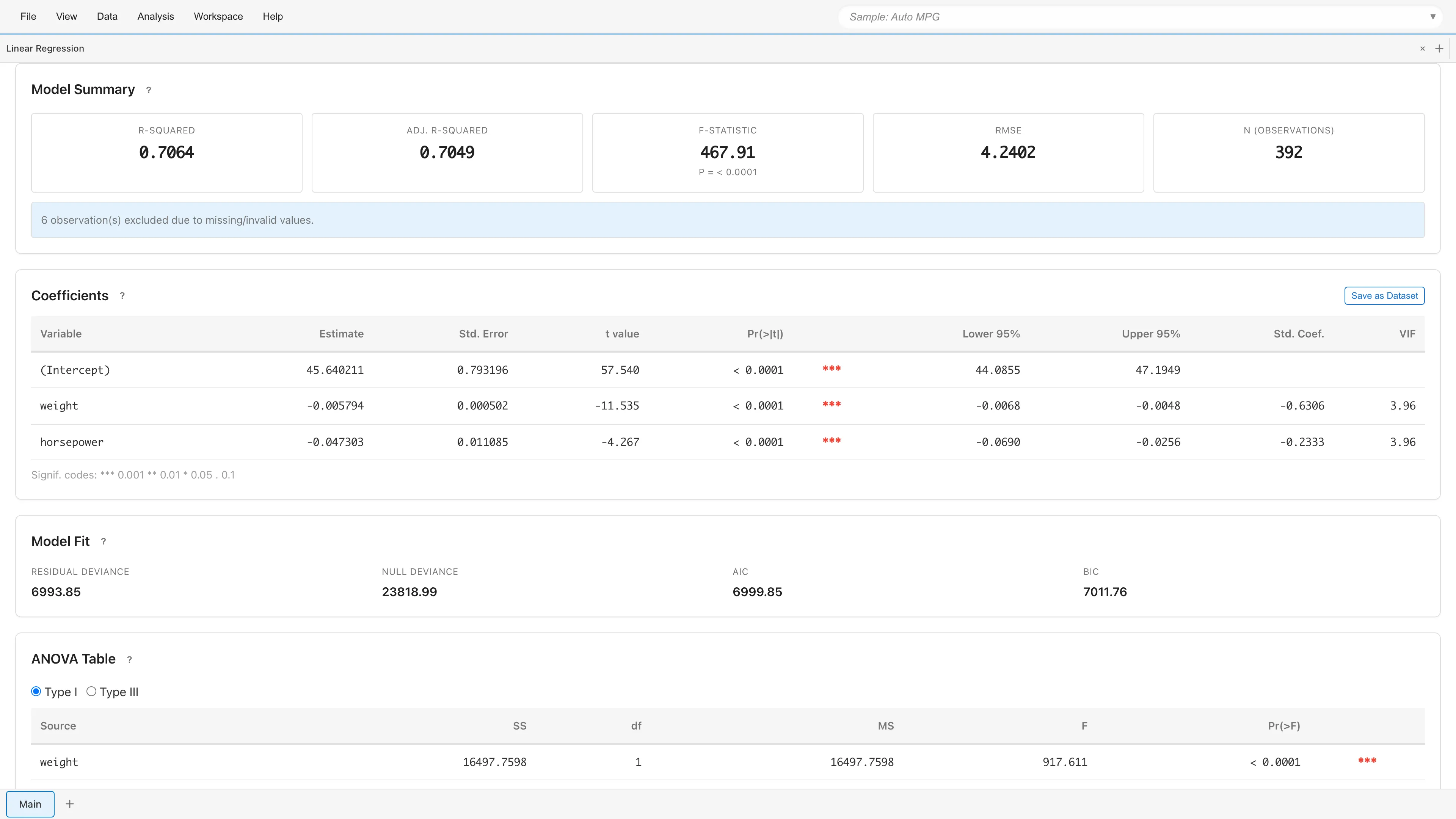
Displays overall model fit statistics.

Metric	Description
R-squared	Proportion of variance explained by the model (0 to 1)
Adj. R-squared	R-squared adjusted for the number of predictors
F-statistic	Overall model significance test (with p-value)
RMSE	Standard deviation of residuals (measure of prediction error)
N (observations)	Number of observations used in the analysis

If rows containing missing or invalid values were excluded, the number of excluded rows is displayed.

Coefficients

Displays regression coefficients and test results for each variable.

Column	Description
Variable	Variable name (intercept shown as "(Intercept)")
Estimate	Estimated coefficient $\hat\beta$
Std. Error	Standard error $\sqrt{\operatorname{diag}\bigl(\hat\sigma^2 (X'X)^{-1}\bigr)}$
t value	$t$ -statistic $t = \hat\beta / \operatorname{SE}(\hat\beta)$ , following a $t_{n-p}$ distribution
Pr(>\|t\|)	Two-sided p-value from the $t$ distribution
(Significance marks)	* p<0.001, p<0.01, * p<0.05, . p<0.1
Lower 95% / Upper 95%	95% confidence interval $\hat\beta \pm t_{\alpha/2,\, n-p} \times \operatorname{SE}(\hat\beta)$
Std. Coef.	Standardized coefficient $\hat\beta_j \times s_{X_j} / s_Y$ for comparing effect sizes across variables (N/A for intercept)
VIF	Variance Inflation Factor (see Multicollinearity)

Under normal errors, the OLS $t$ -test is exact regardless of sample size.

The coefficients table can be saved as a dataset using the Save as Dataset button for export to CSV.

Interpreting Coefficients

Coefficients are directly interpretable on the response scale.

Continuous predictor: Holding other variables constant, a one-unit increase in $X_j$ changes $E[Y]$ by $\hat\beta_j$
Dummy variable: Represents the difference in $E[Y]$ relative to the reference category
Intercept: $E[Y]$ when all predictors are zero
Standardized coefficient (Std. Coef.): Expressed in standard deviation units, enabling direct comparison of effect sizes across variables with different scales

Model Fit

Metric	Description
Residual Deviance	Residual sum of squares $\text{RSS} = \sum(y_i - \hat y_i)^2$
Null Deviance	Total sum of squares $\text{TSS} = \sum(y_i - \bar y)^2$
AIC	Akaike Information Criterion $\text{AIC} = -2\ell + 2p$ . Lower is better
BIC	Bayesian Information Criterion $\text{BIC} = -2\ell + p \ln n$ . Penalizes complexity more strongly than AIC

ANOVA Table

ANOVA table

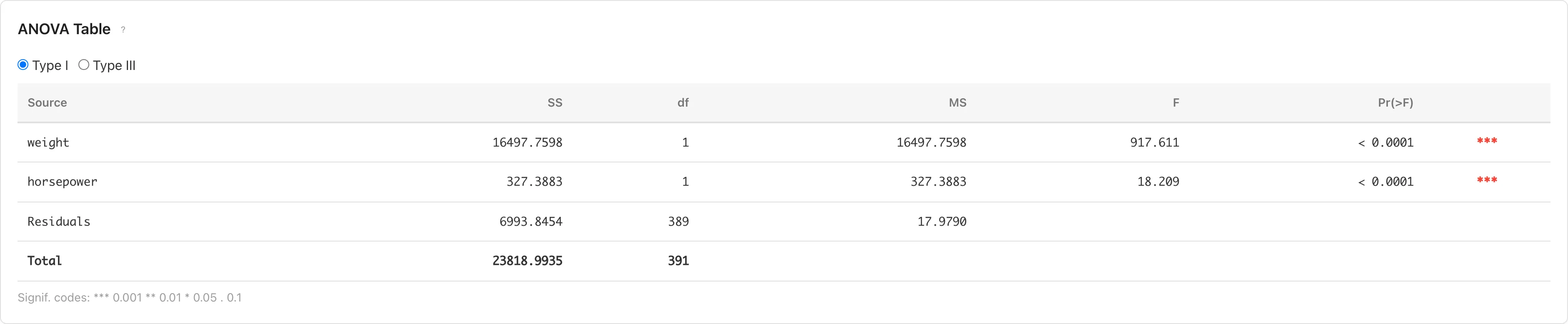
Evaluates each predictor's contribution through analysis of variance. Switch between Type I and Type III using radio buttons.

Type I (Sequential): Computes sum of squares in the order variables were entered. Results depend on variable entry order.
Type III (Partial): Computes sum of squares as if each variable were entered last. Results are independent of variable entry order.

Column	Description
Source	Source of variation
SS	Sum of squares
df	Degrees of freedom
MS	Mean square (SS / df)
F	F-statistic (MS / MS_Residual)
Pr(>F)	p-value based on the F distribution

Prediction & Confidence Intervals

Displays predicted values and interval estimates for each observation.

Column	Description
Obs	Observation number
Fitted	Predicted value
95% CI Lower / Upper	95% confidence interval for the mean response
95% PI Lower / Upper	95% prediction interval for individual observations

The confidence interval (CI) represents the precision of the estimated mean, while the prediction interval (PI) represents the range for a new individual observation. PI is always wider than CI. The confidence level is fixed at 95%.

When exceeding 100 rows, only the first 50 rows are displayed. Click Show all N rows to display all rows.

Saving and Diagnostics

Model saving

Save analysis results to the project and view diagnostic plots.

Saving the Model

Enter a model name in the Model Name field and click Save Model. The model name defaults to the format "Linear Regression: Y ~ X1 + X2".

If an existing model with the same configuration (dataset, response variable, predictor variables) exists, a confirmation dialog for overwriting is displayed.

Data Generated on Save

Saving a model automatically creates a derived dataset that adds diagnostic columns to the original data.

Column	Symbol	Description
`fitted_values`	$\hat y_i$	Predicted values
`deviance_residuals`	$e_i = y_i - \hat y_i$	Residuals
`standardized_residuals`	$r_i^* = e_i / (\hat\sigma\sqrt{1 - h_i})$	Standardized residuals
`leverage`	$h_i$	Leverage (diagonal of the hat matrix)
`cooks_distance`	$D_i$	Cook's Distance

Diagnostics and Details

After saving the model, two buttons appear:

View Model Details - Opens the Model Detail tab showing detailed model information
View Diagnostics - Opens the Residual Diagnostics tab showing residual diagnostic plots

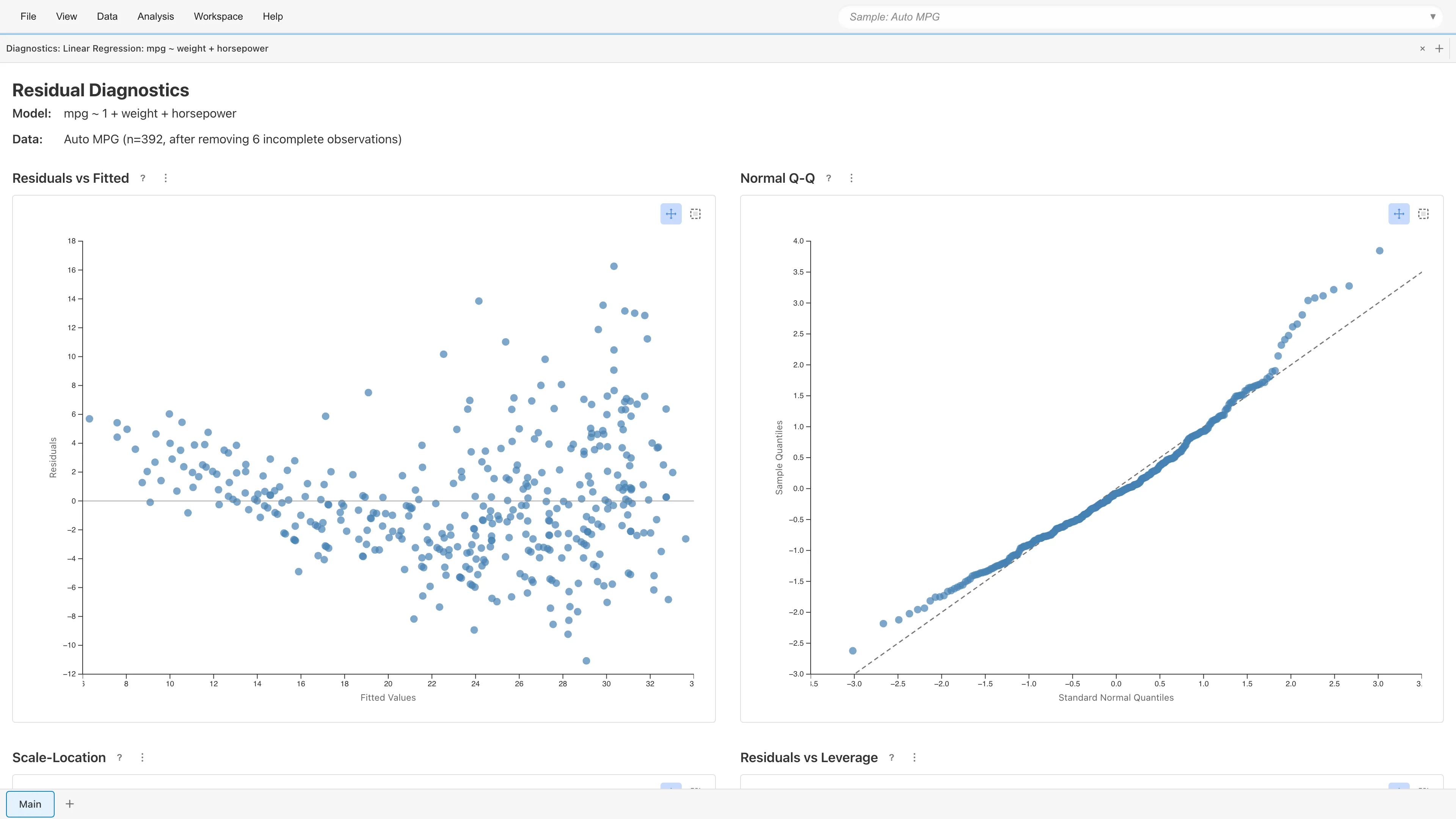
Residual Diagnostics

View Diagnostics opens four diagnostic plots for assessing the OLS assumptions:

OLS assumptions:

Linearity - A linear relationship exists between the response and predictor variables
Normality - Residuals follow a normal distribution
Homoscedasticity - The variance of residuals is constant and does not depend on fitted values
Independence - Residuals are independent of each other (not directly verifiable through diagnostic plots). For hierarchical or clustered data, consider using GLMM with random effects. MIDAS does not currently support time series autocorrelation

Residual diagnostics

The diagnostic plots use standardized residuals $r_i^*$ . See Regression Analysis Fundamentals for the formulas.

Residuals vs Fitted

Plots residuals $e_i$ against fitted values $\hat y$ . With a well-specified model, residuals scatter randomly around zero.

Curved pattern: Nonlinear effects of predictors may be missing
Funnel-shaped pattern: Possible heteroscedasticity (check Scale-Location plot for details)

Normal Q-Q Plot

Plots standardized residual $r_i^*$ quantiles against theoretical normal quantiles. Points fall along the diagonal when residuals are normally distributed. Deviation at both ends indicates heavy tails; an S-shaped departure indicates skewness.

Scale-Location

Plots $\sqrt{|r_i^*|}$ against fitted values. Constant variance produces an even horizontal spread. A funnel-shaped or upward-trending pattern indicates heteroscedasticity. When heteroscedasticity is present, coefficient estimates remain unbiased but standard errors become inaccurate, making confidence intervals and p-values unreliable.

Residuals vs Leverage

Plots standardized residuals $r_i^*$ against leverage $h_i$ . Cook's (1977) distance contours ( $D = 0.5$ : orange dashed, $D = 1.0$ : red dashed) are overlaid. Cook suggested comparing $D_i$ to the 50th percentile of $F_{p,\, n-p}$ , which is typically near 1. This is not a formal rejection threshold but a guide for comparing relative influence among observations.

Leverage: Measures how far an observation's predictor values are from others. $2p/n$ is the conventional threshold for high leverage
Cook's Distance: Combines leverage and residual size into a single influence measure

Observations outside the contour lines may substantially change the model estimates if removed.

Point Selection

Click or rectangle-select data points on any plot to display details (fitted values, residuals, leverage, Cook's Distance, etc.) in a table below the plots. Selection state is synchronized across all four plots.

Notes

Using Categorical Variables

OLS regression only accepts numeric variables. To use string or boolean categorical variables as predictors, convert them to numeric dummy variables using the Dummy Coding tab before running the analysis.

Automatic Exclusion of Missing and Invalid Values

Rows containing missing values (null), non-numeric values, or infinity are automatically excluded from the analysis. The number of excluded rows is displayed in the Model Summary.

Multicollinearity

When predictors are highly correlated, coefficient estimates become unstable. If VIF (Variance Inflation Factor) is large for any variable in the coefficients table, consider removing redundant variables or combining correlated predictors. See Regression Analysis Fundamentals for details on VIF.

Sample Size and Normality

The finite-sample exactness of $t$ -tests and $F$ -tests depends on the normality of errors. With large samples, the central limit theorem ensures the test statistics are approximately normal, but for small samples, verify residual normality using the Q-Q plot. The required sample size depends on the true error distribution, so no universal threshold applies.

References

Cook, R. D. (1977). Detection of influential observation in linear regression. Technometrics, 19(1), 15-18.

Next steps

Residual Diagnostics - Verify model assumptions
Generalized Linear Model (GLM) - Modeling count data and binary outcomes